Bernhard Holzer

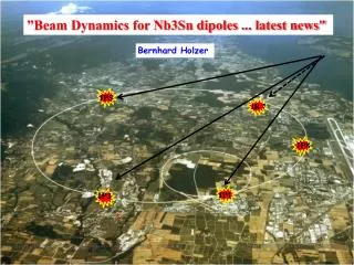
1. ”Beam Dynamics for Nb3Sn dipoles ... latest news" Bernhard Holzer IP5 IR 7 IP8 IP1 IP2 *

2. DS Upgrade Scenarios halo Shift 12 Cryo-magnets, DFB, and connection cryostat in each DS transversely shifted by 4.5 cm halo New ~3..3.5 m shorter Nb3Sn Dipoles (2 per DS) -4.5m shifted in s +4.5 m shifted in s M. Karppinen TE-MSC-ML

3. Effects to be expected: * magnets are shorter than MB Standards change of geometry distortion of design orbit * R-Bends  S-Bends  edge focusing distortion of the optics tune shift, beta beat * nonlinar transfer function (3.5 TeV)  distortion of closed orbit to be corrected locally ?? dedicated corrector coils ?? trim power supply ?? * feed down effects from sagitta ? * multipole effect on dynamic aperture ? Sixtrack Tracking Simulations

4. Problem 1.) Influence on Optics: Edge FocEffect optics distortion beta beat: tune shift: Problem 2.) Influence on Optics: Sagitta & Feed Down Influence on Optics and Aperture are quite limited

5. Problem 3.) Feed Down Effects: first error estimates: b3 =108 units Quadrupole Error: Tuneshift: Beta Beat considered as tolerance limit (DA) per Magnet

6. Problem 1: “non-linear” Transfer Function Below Inom 11 T Dipole is stronger than MB M. Karppinen CERN TE-MSC-ML

7. The Story of the Transfer Function ... a closed orbit problem calculate the ideal (nb3sn) machine flatten the experiment bumps, switch off LHC-B, ALICE etc assign field error to nb3sn dipoles correct the orbit plot the residual error what are we talking about ... treated not as a geometrical problem but as a orbit problem  to be corrected.

8. ... 10 seconds for the contemplation: Nb3Sn Transferfunction: worst case (... around 3.5 TeV) = 2.7% lack in main field rough estimate: Δx ≈ 13 mm source of the problem: orbit correctors are located at the quadrupoles, with a cell length of 105m. Q8 Q9 Q10

9. 4.) The Story of the Transfer Function ... a closed orbit problem effect of nb3sn field error (1.5 Tm) two dipoles distorted orbit, and corrected by the “usual methods” x(m) x(m) Δx ≈ -0.5 ... + 1.5 mm  ≈ 5 σ at 3.5 TeV two Nb3Sn magnets corrected by 20 orbcor dipoles

10. 4.) The Story of the Transfer Function ... a closed orbit problem field error corrected by 3 (20) most eff. correctors zooming the orbit distortion ... local distortion due to Δϕ ≈ 4.545 phase relation, closed by MCBH correctors Δs=500m ! MCBH corrector strength: available: 1.900 Tm needed: 0.805 Tm = 42 %

11. New RB Circuit (Type 1) Trim2 C8 C9 C10 C11 C8 0.15H RB.A23 0.1H Trim1 Main Power Converter TRIM Power Converters Total inductance: 15.5 H (152x0.1H + 2x0.15H) Total resistance: 1mW Output current: 13 kA Output voltage: 190 V Total inductance: 0.15 H Total resistance: 1mW RB output current: ±0.6 kA RB output voltage: ±10 V • (+) • Low current CL for the trim circuits • Size of Trim power converters • (-) • Protection of the magnets • Floating Trim PCs (>2 kV) • coupled circuits Courtesy of H. Thiessen

12. Problem 2: Multipole Errors & Dynamic Aperture in Nb3Sn Dipoles ... the very first estimates ... in the usual units, i.e. 10 -4 referred to the usual ref radius = 17mm

13. Nb3Sn Dipole: Multipole Errors: ... the very first estimates

14. NbTi Dipole: Multipole Errors:

15. the persistent current problem: tracking studies needed M. Karppinen CERN TE-MSC-ML

16. Where are we ? IP1,2,5,IP7 Q8 Q9 Q10 Present Option: 2 x 5.5m Nb3Sn Dipoles separated

17. optics situation collision optics, 7 TeV

18. Tracking Studies: Dynamic Aperture determined via stability / survival time theory: phase space ellipse defined by optical parameters ideal, linear machine strong b3 multipole Phase Space Distance b3 = 98, full & local correction b3 = 98, no correction

19. Tracking Studies: Dynamic Aperture determined via survival time b3 = 98, no correction survival time ... measured in number of turns ... gives an indication of the influence of the non-linear fields on the ( an- ) harmonic oscillation of the particles. y For the experts: 60 seeds, 10^5 turns, 4-18 σ in units of 2, 30 particle pairs, 17 angles x

20. Field Quality: Dynamic Aperture Studies 7 TeV Case, luminosity optics (55cm) ε=5*10-10 radm ( εn= 3.75μm) ideal Nb3Sn dipoles mult. coeff. à la error table6 at high field the higher harmonics are small enough, the p.c. effects disappeared and the emittance is reduced (Liouville)

21. Field Quality injection optics, 450 GeV two options: 1.) introduce a strong local spool piece corrector to accept the large b3 2.) set tolerance limits to b3 to compensate with the standard “mcs” dyn aperture injection optics, average of 60 seeds Option 1.) ideal Nb3Sn magnets (an=bn=0) an=bn=Nb3Sn values but b3 = 0 b3=full, local compensation b3 =full, no correction for the experts: if b3 is corrected locally the Nb3Sn behave like (nearly) ideal magnets Higher order multipoles do not have a strong influence on the DA A strong mcs like compensator is needed at every Nb3Sn.

22. Option 1.) accept the large b3 and install a local correction Standard MCS: l = 110 mm g2 = 1630 T/m2 Standard pc contribution: NbTib3 = 7.9 units pc contribution: Nb3Sn b3 = 108 units, compensation via MCS: k2 l = 0.412 /m2 g2 = 5618 T/m2 ... without snap back contribution ? what about higher multipoles ?? what about the skews ??? what about reality

23. Option 2.) determine tolerance limits for the b3 at injection ... and try to improve the technical design dyn aperture injection optics, minimum of 60 seeds dynamic aperture for Nb3Sn case: full error table (red) b3 reduced to 50% (green) b3 reduced to 25% (violett) b3 = 0 and to compare with: present LHC injection for the experts: there is not much difference between b3=0 and perfect Nb3Sn magnets !! A scan in b3 values has been performed and shows that values up to b3 < 20 units are ok.

24. Field Quality: First Prototype Injection Optics, 450 GeV, first measured values: “FNAL-demo-2” and again the tracking ... systematics -> FNAL prototype random -> best guess uncertainty - > MB standard dipole ideal Nb3Sn dipoles, an=bn=0 first FNAL prototype systematics & Mikkos random artificially enhanced b4...6 , a3 first measured values are just at the limit but at the moment in sufficient dynamic aperture is obtained.

25. 2, 6, 8, 10, 12 pol skew & trim quad, chroma 6pol, landau 8 pole LHC: Basic Layout of theMachine FoDo and multipolecorrectormagnets MCS ! ----------------------------------------------------------------------- ! ********Magnet type : MQXC/MQXD (new Inner Triplet Quad)*************** ! ----------------------------------------------------------------------- bn in collision b1M_MQXCD_col := 0.0000 ; b1U_MQXCD_col := 0.0000 ; b1R_MQXCD_col := 0.0000 ; b2M_MQXCD_col := 0.0000 ; b2U_MQXCD_col := 0.0000 ; b2R_MQXCD_col := 0.0000 ; b3M_MQXCD_col := 0.0000 ; b3U_MQXCD_col := 0.4600 ; b3R_MQXCD_col := 0.8900 ; b4M_MQXCD_col := 0.0000 ; b4U_MQXCD_col := 0.6400 ; b4R_MQXCD_col := 0.6400 ; b5M_MQXCD_col := 0.0000 ; b5U_MQXCD_col := 0.4600 ; b5R_MQXCD_col := 0.4600 ; b6M_MQXCD_col := 0.0000 ; b6U_MQXCD_col := 1.7700 ; b6R_MQXCD_col := 1.2800 ; b7M_MQXCD_col := 0.0000 ; b7U_MQXCD_col := 0.2100 ; b7R_MQXCD_col := 0.2100 ; b8M_MQXCD_col := 0.0000 ; b8U_MQXCD_col := 0.1600 ; b8R_MQXCD_col := 0.1600 ; b9M_MQXCD_col := 0.0000 ; b9U_MQXCD_col := 0.0800 ; b9R_MQXCD_col := 0.0800 ; b10M_MQXCD_col := 0.0000 ; b10U_MQXCD_col := 0.2000 ; b10R_MQXCD_col := 0.0600 ; b11M_MQXCD_col := 0.0000 ; b11U_MQXCD_col := 0.0300 ; b11R_MQXCD_col := 0.0300 ; b12M_MQXCD_col := 0.0000 ; b12U_MQXCD_col := 0.0200 ; b12R_MQXCD_col := 0.0200 ; b13M_MQXCD_col := 0.0000 ; b13U_MQXCD_col := 0.0200 ; b13R_MQXCD_col := 0.0100 ; b14M_MQXCD_col := 0.0000 ; b14U_MQXCD_col := 0.0400 ; b14R_MQXCD_col := 0.0100 ; b15M_MQXCD_col := 0.0000 ; b15U_MQXCD_col := 0.0000 ; b15R_MQXCD_col := 0.0000 ; multipole correction chrom correction orbit correction

27. Field Quality: Second Prototype Injection Optics, 450 GeV Sec 2/7, min values second prototype gives better DA than the first prototype ... and considerably better DA than the b3 tolerance limit

28. Field Quality: Second Prototype Nb3 Sn in different sectors Injection Optics, 450 GeV, standard mcscorreection, second prototype different sectors: #2, #2/7, #1,2,5 min values different sectors: #2, #2/7, #1,2,5 min values As long as standard mcs compensation is used, the number of sectors is not very relevant

29. Field Quality: Second Prototype, no mcs ??? can we remove the standard mcs ??? ... a dangerous approach ... One sector, compare Sec 2 with / without mcs scaled and not “scaled” => increase the mcs in the corresponding sector by 154/152 mcs mcs scaled no mcs removing mcs dos not improve the situation scaled or un-scaled.

30. Field Quality: Second Prototype, no mcs ??? can we remove the standard mcs ??? ... a dangerous approach ... Different sectors, compare sec #2 sec #2,7 sec #1,2,5 sec #1,2,5 with scaled mcs correction (avg). As long as we stay within the tolerance limits for the second prototype a correction of the b3 seems possible if the remaining mcs are scaled up.

31. Resume: Nb3Sn dipoles in the cold collimation part have (nearly) no effect on the beam optic have (nearly) no effect on the LHC global geometry local geometry has to be discussed have a strong influence on the orbit that can be corrected outside the dipole pair using a considerable fraction of the available corrector strength a relatively large orbit distortion (5σ) remains between the dipole pairs Installation trim power supply to compensate seems the ideal solution Multipoles are an issue: driving problem: b3 They have only small impact at high energy, At 450 GeV injection they were too strong in first field estimates they could however be reducedconsiderably in the 2nd prototype The b3 has – and can - to be compensated by the mcs standard spool pieces A correction scheme without local mcs seems possible, leads however in some cases to a reduced DA.