Download
1 / 64
650 likes | 837 Vues
Uncertainty Handling in Bayesian Network CS570 Lecture Note by Jin Hyung Kim Computer Science Department, KAIST jkim@kaist.ac.kr. Compiled from - Bayesian Networks without Tears, Eugene Charniak, AI Magazine, Winter 1991, pp.50~63 - Lecture note by Jeong-Ho Chang, SNU

E N D
Uncertainty Handling in Bayesian Network CS570 Lecture Note by Jin Hyung Kim Computer Science Department, KAIST jkim@kaist.ac.kr Compiled from - Bayesian Networks without Tears, Eugene Charniak, AI Magazine, Winter 1991, pp.50~63 - Lecture note by Jeong-Ho Chang, SNU - Lecture note by KyuTae Cho ,Jeong Ki Yoo ,HeeJin Lee, KAIST
Reasoning Under Uncertainty • Motivation • Truth value is unknown • Too complex to compute prior to make decision • characteristics of real-world applications • Source of Uncertainty • cannot be explained by deterministic model • decay of radioactive substances • Don’t understand well • disease transmit mechanism • Too complex to compute • coin tossing
Types of Uncertainty • Randomness • Which side will be up if I toss a coin ? • Vagueness • Am I pretty ? • Confidence • How much do you confident on your decision ? • Degree of Belief • The sentence itself is in fact either true or false • Same ontological commitment as logic ; the facts either do or do not hold in the world • Probability theory • Degree of Truth (membership) • Not a question of the external world • Case of vagueness or uncertainty about the meaning of the linguistic term “tall”, “pretty” • Fuzzy set theory, fuzzy logic One Formalism for all vs. Separate formalism Representation + Computational Engine
Representing Uncertain Knowledge • Modeling • select relevant (believed) propositions and events • ignore irrelevant, independent events • quantifying relationships is difficult • Consideration of Representation • problem characteristic • degree of detail • Computational complexity • simplification by assumption • Data is obtainable ? • Computational Engine is available ?
Uncertain Representation Binary Logic Multi-valued Logic Probability Theory Upper/Lower Probability Possibility Theory 1 0
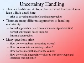
Why First-order Logic Fails? • Laziness : Too much works to prepare complete set of exceptionless rule, and too hard to use the enormous rules • Theoretical ignorance : Medical science has no complete theory for the domain • Practical ignorance : All the necessary tests cannot be run, even though we know all the rules
Probabilistic Reasoning System • Assign probability to a proposition based on the percepts that it has received to date • Evidence : perception that an agent receives • Probabilities can change when more evidence is acquired • Prior / unconditional probability : no evidence at all • Posterior / conditional probability : after evidence is obtained
Uncertainty and Rational Decisions • No plan can guarantee to achieve the goal • To make choice, agent must have preferences between the different possible outcomes of various plans • missing plane v.s. long waiting • Utility theory to represent and reason with preferences • Utility: the quality of being useful (degree of usefulness) • Decision Theory = Probability Theory + Utility Theory • Principle of Maximum Expected Utility : An agent is rational if and only if it chooses the action that yields the highest expected utility, average over all possible outcomes of the action
Applications involving Uncertainty • Wide range of Applications • diagnose disease • language understanding • pattern recognition • managerial decision making • useful answer from uncertain, conflicting knowledge • acquiring qualitative and quantitative relationships • data fusion • multiple experts’ opinion
Probability Theory • Frequency Interpretation • flipping coin • generalizing future event • Subjective Interpretation • Probability of your passing in the national exam • degree of belief
Basic Probability • Prior probability P(A) : unconditional or prior probability that the proposition A is true • Conditional Probability • P(a|b) = P(a,b)/P(b) • Product rule -> P(a,b)P(b) • The axioms of Probability (Kolmogorov’s axioms) • 0<= P(a) <= 1, for any proposition a • P(true) =1 , P(false) = 0 • P(a٧b) = p(a)+p(b) – p(a,b)
Degree of Belief • Elicitation of degree of belief from subject • Agent can provide degree of belief for sentence • lottery - utility functions • Main tool : Probability theory • assign a numerical degree of belief between 0 and 1 to sentences • the way of summarizing the uncertainty that comes from laziness and ignorance • Elicitation of Conditional probability • conversion using Bayes Rule • Different subjective probability to same proposition • due to different background and knowledge $1 $1 0.9 Rain >< 0.1 $0 No Rain $0
Human Judgement and Fallibility A B A or ? B • Systematic bias in probability judgement • Psychologist Tversky’s experiment • conservative in updating belief • A: 80% chance of $4000 • B: 100% chance of $3000 • C: 20% chance of $4000 • D: 25% chance of $3000 A or B ?, C or D ? • Risk-averse with high prob. And risk-taking with low prob.
Random Variable • Variable takes value from sample space • mutually exclusive, exhaustive events • Joint Sample Space x1x2 …. xn = • 0 Pr(X = x) 1, xx and • 1 =
Basic Probability • The probability of a proposition is equal to the sum of the probabilities of the atomic events in which it holds • P(a) = • where e(a) is set of all the atomic events in which a holds • Marginalization, summing out • P(Y) = P(Y,z) • Conditioning • P(Y) = P(Y|z)P(z) • independence between a and b • P(a|b) = P(a) • P(b|a) = P(b) • P(a,b) = P(a)P(b)
More on Probability Theory • Joint Distribution • Probability of co-occurrence • Specifying joint distribution of n variables • require 2n numbers • Conditional Probability • Prior Belief + New evidence Posterior Belief
Calculus of Combining Probabilities • Marginalizing • Addition Rule • Chain Rule Pr(X1, …, Xn) = Pr(X1|X2, …, Xn) Pr(X2|X3, …, X4) …. Pr(Xn-1|Xn) Pr(Xn) • factorization
Bayes Rule • Allows to covert Pr(A|B) to P(B|A), vice versa • Allows to elicit psychologically obtainable values • P( symptom | disease ) vs P(disease | symptom) • P(cause | effect ) vs P(effect | cause ) • P( object | attribute) vs P(attribute | object ) • Probabilistic Reasoning Bayesian School
Conditional Independence • Specifying distribution of n variables • require 2**n numbers • Conditional Independence Assumption • Pr(A|B, C) = Pr(A|C) • A is conditionally independent of B given C • A not depend on B given C We can ignore B in inferring A if we have C • Pr(A,B|C) = Pr(A|C)Pr(B|C) • Chain rule and conditional independence together saves storage • ex : Pr(A,B,C,D) = Pr(A|B)Pr(B|C)Pr(C|D)P(D)
Problems • Approximate the joint probability distribution of n variables by set of 2nd order joint probabilities Pr(ABCD) = P(A)P(B|A)P(C|A)P(D|C) or P(B)P(B|A)P(C|B)P(D|C) or ….. • From P(A) and P(B), estimate P(A, B). • Maximum Entropy Principle
Maximum Entropy Principle • General method to assign values to probabilitydistributions on the basis of partial information • While consistent with given information, probability distribution P is determined as the one that maximize the uncertainty measure H(P). • Choose the Most unbiased one • No reason to favor any one of the propositions over the others • Example • What is P(P= true) for binary random variable P ? • You know P(a) = 0.5 and P(~a) = 0.5, p(b) =0.6, P(~b)=0.4. What is P(a,b) ?
Estimation of High-Order Joint Probabilities • High order joint probability is approximated by Products of lower order probabilities(Lewis 1968) Ex) P(A, B, C) can be approximated by P(A)P(B|A)P(C|A), P(B)P(A|B)P(C|B), P(C)P(A|C)P(B|C) • Selecting best 2nd order product estimation(Chow tree) • Maximum Spanning tree of a graph labeled by mutual information X sj si sk
Mutual Information • Strength of dependencymutual information • Entropy of variable • Conditional Entropy • Mutual information among strokes [Shannon]
Maintaining Consistency • Pr(a|b) = 0.7, Pr(b|a) = 0.3, Pr(b) = 0.5 • inconsisent • check by Bayes rule Pr(a,b) = Pr(b|a)Pr(a) = Pr(a|b)Pr(b) Pr(a) = Pr(a|b)Pr(b) / Pr(b|a) = 0.7 x 0.5 / 0.3 > 1.0
naive Bayes model • a single cause directly influences a number of effects, all of which are conditionally independent, given cause. • P(Cause,Effect1,..., EffectN) = P(Cause)P(Effect1|Cause)... P(EffectN|Cause) • Naive because it is often used in cases where the ‘effect’ variables are not conditionally independent given cause variable. • Though work surprisingly well in practice
Probabilistic Networks • Bayesian Network, Causal Network, Knowledge map • Graphical model of causality and influence • directed acyclic graph, G = (V, E) • V : random variable • E : dependencies between random variables • only one edge connecting two nodes directly • direction of edge : causal influence • for X Y Z • evidence regarding X : causal support of Y • evidence regarding Z : diagnostic support of Y
Bayesian Networks • A compact representation of a joint probability of variables on the basis of the concept of conditional independence. • Qualitative part: graph theory • Directed acyclic graph • Nodes: Random variables • Edges: dependency or influence of a variable on another. • Quantitative part: probability theory • Set of conditional probabilities for all variables • Naturally handles the problem of complexity and uncertainty.
Bayesian Networks (Cont’d) • BN encodes probabilistic relationships among a set of objects or variables. • Model for representing uncertainty in our knowledge • Graphical model of causality and influence • Representation of the dependencies among random variables • It is useful in that • dependency encoding among all variables: Modular representation of knowledge. • can be used for the learning of causal relationships helpful in understanding a problem domain. • has both a causal and probabilistic semantics can naturally combine prior knowledge and data. • provide an efficient and principled approach for avoiding overfitting data in conjunction with Bayesian statistical methods.
BN as a Probabilistic Graphical Model E D C A B Graphical model undirected graph directed graph Markov Random Field Bayesian Networks E D C A B
Representation of Joint Probability E E D C D C A B A B Z3 Z2 Z1 normalization constant
MINVOLSET KINKEDTUBE PULMEMBOLUS INTUBATION VENTMACH DISCONNECT PAP SHUNT VENTLUNG VENITUBE PRESS MINOVL FIO2 VENTALV PVSAT ANAPHYLAXIS ARTCO2 EXPCO2 SAO2 TPR INSUFFANESTH HYPOVOLEMIA LVFAILURE CATECHOL LVEDVOLUME STROEVOLUME ERRCAUTER HR ERRBLOWOUTPUT HISTORY CO CVP PCWP HREKG HRSAT HRBP BP • Joint probability as a product of conditional probabilities • Can dramatically reduce the parameters for data modeling in Bayesian networks. 37 variables in total 509 parameters 254 (From NIPS’01 tutorial by Friedman, N. and Daphne K.)
Real World Applications of BN • Intelligent agents • Microsoft Office assistant: Bayesian user modeling • Medical diagnosis • PATHFINDER (Heckerman, 1992): diagnosis of lymph node disease commercialized as INTELLIPATH (http://www.intellipath.com/) • Control decision support system • Speech recognition (HMMs) • Genome data analysis • gene expression, DNA sequence, a combined analysis of heterogeneous data. • Turbocodes (channel coding) • … • …
Causal Networks Fuel Clean Spark Plugs Fuel Meter Standing Start • Node: event • Arc: causal relationship between two nodes • A B: A causes B. • Causal network for the car start problem [Jensen 01]
Reasoning with Causal Networks Fuel Clean Spark Plugs Fuel Meter Standing Start • My car does not start. increases the certainty of no fuel and dirty spark plugs. increases the certainty of fuel meter’s standing for the empty. • Fuel meter stands for the half. decreases the certainty of no fuel increases the certainty of dirty spark plugs.
d-separation Connections in causal networks C A B A C B A B C Serial diverging converging Definition [Jensen 01]: • Two nodes in a causal network ared-separated if for all paths between them there is an intermediate node V such that • the connection is serial or diverging and the state of V is known or • the connection is converging and neither V nor any of V’s descendants have received evidence.
d-separation (Cont’d) C A B A C B A B C C A B A C B A B C A and B is marginally dependent A and B is marginally independent A and B is conditionally independent A and B is conditionally dependent
d-separation: Car Start Problem Fuel Clean Spark Plugs Fuel Meter Standing Start • ‘Start’ and ‘Fuel’ are dependent on each other. • ‘Start’ and ‘Clean Spark Plugs’ are dependent on each other. • ‘Fuel’ and ‘Fuel Meter Standing’ are dependent on each other. • ‘Fuel’ and ‘Clean Spark Plugs’ are conditionally dependent on each other given the value of ‘Start’. • ‘Fuel Meter Standing’ and ‘Start’ are conditionally independent given the value of ‘Fuel’.
Path-Based Characterization of Independence • A is dependent of C given B • F is independent of D given E B C A E F D
Direction dependent separation (D-separation) • A path P is blocked given set of node E if ZP for which 1. ZE and Z has one arrow in and one arrow out on P 2. ZE and Z has both path arrows out 3. ZE and successor(Z)E, and both path arrows lead to Z • A set of nodes E d-separates two sets of nodes X and Y if every undirected path from X to Y is blocked • If every undirected path from X to Y is d-separable by E, then X and Y are conditionally independent given E.
Z (1) (2) Z E (3) Z Y X Path X to Y is blocked, given evidence E
H : hardware problem B : bug’s in LISP code E : editor is running L : LISP Interpreter O.K. F : Cursor is flashing P : prompt displayed W : dog is barking H W B E L Parent child successor F P
Alarm Example Burglary Earthquake Alarm MaryCalls JohnCalls
Independent relationship • Each node is CI of all non-successors given Parent • Pr(P|E,F,L,J,B,H) = Pr(P|L) • Topological sort of variables • variable after all children • Let X1, X2, …, Xn be a topological sort of variables of G • Pr(Xi | Xi+1, Xi+2, …, Xn) = Pr (Xi | parent(Xi))
H B D C S E L Pr(P,F,L,E,B,H) = Pr(P|F,L,E,B,H)Pr(F|L,E,B,H) Pr(L|E,B,H)Pr(E|B,H)Pr(B|H)Pr(H) = Pr(P|L)Pr(F|E)Pr(L|H,B)Pr(B)Pr(H) F P
Bayesian Networks: Revisited • Definition • A graphical model for the probabilistic relationships among a set of variables. • Compact representation of joint probability distributions on the basis of conditional probabilities. • Consists of the following. • A set of n variables X = {X1, X2, …, Xn} and a set of directed edges between variables. • The variables (nodes) with the directed edges form a directed acyclic graph (DAG) structure. • To each variable Xi and its parents Pa(Xi), there is attached a conditional probability table for P(Xi|Pa(Xi)). • Modeling for the continuous variables is also possible. Qualitative part Quantitative part
Quantitative Specification by Probability Calculus • Fundamentals • Conditional Probability • Product Rule • Chain Rule: a successive application of the product rule.
C A C B • Conditional independence A B A B C • Independence of two events • Marginal independence
Pa(X5): the parents of X4 Ch(X5): the children of X4 De(X5): the descendents of X4 Pa(X5) Topological Sort of Ch(X5) De(X5) X={X1, X2, … , X10} X1 X2 X1, X2, X3, X4, X5, X6, X7, X8, X9, X10 X3 X4 Chain rule in a reverse order X5 X5 X6 X7 X8 X10 X9
Bayesian Networkfor the Car Start Problem P(Fu = Yes) = 0.98 P(CSP = Yes) = 0.96 Fuel Clean Spark Plugs Fuel Meter Standing Start P(FMS|Fu) P(St|Fu, CSP)
Structure(cont.) A B C D E P(a) P(b) P(c|a) P(c|ㄱa) P(d|ab), P(d|aㄱb), P(d|ㄱab), P(d|ㄱaㄱb) P(e|d) P(e|ㄱd) • Initial configuration of BN • Root nodes • Prior probabilities • Nonroot nodes • Conditional probabilities given all possible combinations of direct predecessors