Bayesian Approaches to Image Warping: An Empirical Bayes Framework
This text discusses how empirical Bayes methods can be applied to image warping, particularly focusing on the need to find parameter sets that are maximally likely given the data. It emphasizes the role of Bayesian principles, expressed in the context of likelihood and prior probabilities, for optimizing image registration processes. Additionally, the text highlights the balance between model complexity and effective registration, as well as the use of Expectation-Maximization (EM) algorithms for hyper-parameter estimation, ultimately aiming for improved image warping outcomes.

Bayesian Approaches to Image Warping: An Empirical Bayes Framework
E N D
Presentation Transcript
Image Warping using Empirical Bayes John Ashburner & Karl J. Friston. Wellcome Department of Cognitive Neurology, London, UK.
Bayesian approaches to image warping • Image warping procedures are often thought of as a regularised maximum likelihood problem, and involve finding a set of parameters for a warping model that maximise the likelihood of the observed data. What is actually needed is a set of parameters that are maximally likely given the data. In order to achieve this, the problem should be considered within a Bayesian context, and expressed something like: • “The posterior probability of the parameters given the data is proportional to the likelihood of observing the data given the parameters times the prior probability of the parameters.” P(x|y) P(y|x) P(x) • Taking logs converts the Bayesian problem into one of simultaneously minimising two cost function terms. The first is usually a measure of intensity correlation between the images (likelihood potential), and the second is a measure of the warp roughness (prior potential). • -log P(x|y) = -log P(y|x) + -log P(x) + const Image Warping using Empirical Bayes, Ashburner & Friston, 2001
A generative model for image registration. • Registration (in one dimension) involves minimising something like: • 1 y(n)Ty(n) + 2 x(n)TV-1x(n) • where: yi(n) = gi-f(i+kbik xk(n)) • gi is the ith voxel of the template image. • f(j) is the interpolated value of the source image at point j. • xk(n) is the kth parameter estimate at iteration n. • bik is the ith value of the kth spatial basis function. • At each iteration, x is updated by (Ashburner & Friston, 1999): • x(n+1) = x(n) - (1A(n)TA(n) + 2V-1)-1(1A(n)Ty(n) + 2V-1x(n)) • where: • x(n) are the parameter estimates at iteration n. • y(n) are the current differences between source image and template at iteration n. • A(n) are the derivatives of y(n) with respect to each parameter. • V is the form of the a priori covariance matrix for the parameters. • 1 and 2 are hyper-parameters describing the relative importance of the cost function terms. • The choice of 1 and 2 strongly influences the final solution. Image Warping using Empirical Bayes, Ashburner & Friston, 2001
Getting the right balance • An ongoing argument within the field of image registration is something to the effect of “if there are too many parameters in a registration model, then the model will be over-fitted”, versus “if not enough parameters are used, then the images can not be registered properly”. • A better way of expressing this problem is in terms of obtaining an optimal balance between the cost function terms, which involves assigning the most appropriate weighting to each. • These weights (hyper-parameters 1 and 2in this example) can be estimated using an Empirical Bayes approach, which employs an expectation maximisation (EM) optimisation scheme. • See also abstract #220 (Phillips et al, 2001), which uses Empirical Bayes to determine optimal regularisation for the EEG source localisation problem. Image Warping using Empirical Bayes, Ashburner & Friston, 2001
EM framework • Objective is to find the hyper-parameters (), that maximise the likelihood of observed data (y), given that there are un-observed variables (x) in the model: P(y| ) = xP(y|x, ) dx • Introduce a distribution Q(x) to approximate P(x|y,) . • EM maximises a lower bound on P(y| ) (Neal & Hinton, 1998).. • Lower bound is exact when Kullback-Liebler (KL) divergence between Q(x) and P(x|y,) is zero. • Objective function to maximise is (the free energy): F(Q, ) =log P(y| ) - xQ(x) log (Q(x)/P(x|y,)) dx = xQ(x) log P(x,y|) dx - x Q(x) log Q(x) dx • Expectation Maximisation algorithms maximise F(Q, ): • E-step: maximise F(Q, ) w.r.t. Q keeping constant. • M-step: maximise F(Q, ) w.r.t. keeping Q constant. Image Warping using Empirical Bayes, Ashburner & Friston, 2001
REML objective function • Simple linear generative model: y = Ax + e. where e ~ N(0,C()) • A is MN, MM covariance matrix C() parameterised by . • and x are assumed to be drawn from a uniform distribution, so: P(x,y|) = P(y|x,) = (2)-M/2 |C()|-1/2 exp(-(y-Ax)TC()-1(y-Ax)) • The distributing approximation is: Q(x) = (2)-N/2 |ATC()-1A|1/2 exp(-(x-)ATC()-1A(x-)) • After a bit of rearranging... xQ(x) log P(x,y|)dx = -M log(2) - log|C()| - (y-A)TC()-1(y-A)) - M xQ(x) log Q(x)dx = -N log(2) + log|ATC()-1A| - M • Combining these, the cost function becomes the Restricted Maximum Likelihood (REML) objective function (see e.g., Harville, 1977): F(Q, ) = - log|C()| - (y-A)TC()-1(y-A)) - log|ATC()-1A| + const Image Warping using Empirical Bayes, Ashburner & Friston, 2001
Simple REML estimation. • Consider a simple model: • y = Ax + , where ~N(0, 1I), and x~N(0, 2V) • where A is MxN and V is NxN • The REML objective function for estimating 1 and 2is: • F(Q, ) = M log1 +N log2 - 1(y-Ax)T(y-Ax)- 2xTV-1x+ log|1ATA(n)+2V-1| + const • A straightforwardalgorithm for maximising F(Q, ) is: repeat{ E-step: compute expectation of x by: T = (1(n)ATA + 2(n)V-1)-1 x= T(1(n)ATy + 2(n)V-1x) M-step: re-estimate hyper-parameters (): 1(n+1) = (M - 1(n)tr(TATA))/((y-Ax)T(y-Ax)) 2(n+1) = (N - 2(n)tr(TV-1))/(xTV-1x) } until convergence Image Warping using Empirical Bayes, Ashburner & Friston, 2001
Algorithm for non-linear REML estimation A similar iterative algorithm can be obtained for image registration problems that estimate by maximising the REML objective function. Initialise by assigning starting estimates to x and . Repeat { E-step: compute MAP estimate of parameters (x) by repeating { Compute A(n) from basis functions and gradient of f. yi(n) = gi-f(i+kbik xk(n)) r1 = y(n)Ty(n) r2 = x(n)TV-1x(n) x(n+1) = x(n) - (1A(n)TA(n) + 2V-1)-1(1A(n)Ty(n) + 2V-1x(n)) }… until 1r1+2r2 converges. M-step: re-estimate hyper-parameters (): 1(n+1) = (M - 1(n)tr((1(n)ATA + 2(n)V-1)-1ATA))/r1 2(n+1) = (N - 2(n)tr((1(n)ATA + 2(n)V-1)-1 V-1))/r2 } until M log1 + N log2 - 1r1 - 2r2 + log|1ATA+2V-1| converges Image Warping using Empirical Bayes, Ashburner & Friston, 2001
The problem with smoothness • Images are normally smoothed before registering. • Makes Taylor series approximation more accurate. • Reduces confounding effects of differences that can not be modelled by a small number of basis functions. • Reduces the number of potential local minima. • Unfortunately, the REML model assumes that residuals are i.i.d. after modelling the covariance among the data. • A more robust, but less efficient estimator of the warps is obtained using smoothed images (see Worsley & Friston 1995) • Pure REML is not suitable for this. • Consider: y = Ax + , where ~N(0, 1S), and x~N(0, 2V) • S is autocorrelation among data - e.g. Gaussian. • A more robust estimator: x= (1(n)ATA + 2(n)V-1)-11(n)ATy • A more efficient estimator: x= (1(n)ATS-1A + 2(n)V-1)-11(n)ATS-1y Image Warping using Empirical Bayes, Ashburner & Friston, 2001
Coping with smoothness • Modified algorithm devised that uses the more robust estimator • it appears to work, but we can’t prove why. repeat{ “E-step”: compute robust estimation of x by: T = (1(n)ATA + 2(n)V-1)-1 x= T1(n)ATy “M-step”: re-estimate hyper-parameters (): 1(n+1) = (tr(S-1(n)TATSA))/((y-Ax)TS(y-Ax)) 2(n+1) = (N - 2(n)tr(TV-1))/(xTV-1x) } until convergence • Residual smoothness is likely to differ at the end of each iteration • FWHM of Gaussian smoothing is re-estimated from the residuals before each “M-step” (Poline et al, 1995). • S is computed from this FWHM Image Warping using Empirical Bayes, Ashburner & Friston, 2001
Laplace approximations & residual smoothness • Approximations involve modelling a non-Gaussian distribution with a Gaussian. • Assumes a quadratic form for the errors. • Sum of squares difference is not quadratic with displacement. • Residual variance under-estimates displacement errors for larger displacements. • Partially compensated using a correction derived from estimated smoothness of residuals. • Illustrated by computing sum of squares difference between an image and itself translated by different amounts • this ad hoc correction involves multiplying by square of estimated FWHM of residuals. Image Warping using Empirical Bayes, Ashburner & Friston, 2001
Discussion • Still early days... • Evaluations only on simulated 1D data - appear to work well. • Correction for smoothness may need refining. • Current version works - but don’t know why. • Local minima reduced because the algorithm determines a good balance among the hyper-parameters at each iteration. • Automatically increases model complexity as the fit improves (see e.g., Lester and Arridge, 1999). • The future... • Modifications for non-linear regularisation methods. • More complex models of shape variability using more hyper-parameters. • Better variability estimates by simultaneously registering many images. • Would give a more complete picture of the structural variability expected among a population. This is information that could be used by subsequent image warping procedures in order to make them more accurate. Image Warping using Empirical Bayes, Ashburner & Friston, 2001
References • J. Ashburner and K. J. Friston. “Nonlinear spatial normalization using basis functions”. Human Brain Mapping7(4):254-266, 1999. • D. A. Harville. “Maximum likelihood approaches to variance component estimation and to related problems”. Journal of the American Statistical Association72(358):320-338, 1977. • R. M. Neal and G. E. Hinton. “A view of the EM algorithm that justifies incremental, sparse and other variants”. In Learning in Graphical Models, edited by M. I. Jordan. 1998. • C. Phillips, M. D. Rugg and K. J. Friston. “Systematic noise regularisation for linear inverse solution of the source localisation problem in EEG”. Abstract No. 220. HBM2001, Brighton, UK. • J.-B. Poline, K. J. Worsley, A. P. Holmes, R. S. J. Frackowiak and K. J. Friston. “Estimating smoothness in statistical parametric maps: variability of p values”. JCAT 19(5):788-796, 1995. • K. J. Worsley and K. J. Friston. “Analysis of fMRI time-series revisited - again”. NeuroImage2:173-181, 1995. • H. Lester and S. R. Arridge. “A survey of hierarchical non-linear medical image registration”. Pattern Recognition 32:129-149, 1999. • Matlab code illustrating a simple 1D example is available from: • http://www.fil.ion.ucl.ac.uk/~john/misc • Many thanks to Keith Worsley and Tom Nichols for pointing us to the REML and Empirical Bayes literature, and to Will Penny for many useful discussions. Image Warping using Empirical Bayes, Ashburner & Friston, 2001