Download
1 / 22
220 likes | 361 Vues
Compatibility between, and Merging of, OC data streams. Globcolour first user consultation meeting (Dec. 06, Villefranche-sur-mer) André Morel. OVERVIEW Before merging : Coherency of the various algorithms - The various [Chl] algorithms - The Kd(490) algorithms

E N D
Compatibility between, and Merging of, OC data streams Globcolour first user consultation meeting (Dec. 06, Villefranche-sur-mer) André Morel
OVERVIEW • Before merging: Coherency of the various algorithms • - The various [Chl] algorithms • - The Kd(490) algorithms • After merging: Other Developments and applications • - From near surface [Chl], to the depth of the euphotic layer • - From near-surface [Chl], to the Secchi disk depth • From Kd(490) to Kd(PAR), to the thickness of the heated layer • From {Chl] and geometry, to turbidity-related radiance excess
OC4v4 Differing Algorithms for [Chl] °OC4v4 and OC3Moempirical °OC4Mesemi-analytical (based on a hyperspectral model for Case 1 waters) The same hyperspectral model allows the Derivation of MERIS-type algo. spectrally tuned for the other sensors (other band setting), Such as OC4Me555 -> OC4v4 OC3Me550 -> OC3Mo SeaWiFs OC3Mo MODIS OC4Me MERIS
Same Reflectance ratios (Ri/Rj) are Introduced into OC4v4 and its MERIS-type Counterpart (OC4Me555) and OC3Mo and counterpart (OC3Me550) THEN Compare the [Chl] returns Conclusions: - Small discrepancies When [Chl] < 0.03 And [Chl] > 2 mg/m3 - Agreementfor 95% of the whole ocean Transfer functions (convertibility) available
Kd(490) Algorithms (Newport NASA Workshop April 2006) Curvature (sigmoidal shape) In the relationships between any Ri/Rj and [Chl] Must be present in The relationship between Ri/Rj and Kd(490) Analytically derived relationship (black curve) + NOMAD data This relationship can be used as an algorithm for Kd(490) METHOD 1 (algo OK2-555)
METHOD 1 (Semi-analytical Algo OK2-555) Applied to NOMAD data
(Kd490 = 0.0166 + 0.0835[Chl]^0.633) Method 1 (alg 1.1) and Method 2 (algo 2-2) provide exactly the same results (both are semi-analytical and rest on the same hyperspectral bio-optical model) Methods 1.1 and 2-1 slightly diverge (semi-analytical Kd(490) vs empirical retrieval for Chl)
Kd(490) and [Chl] empirical relationships (Case 1 waters only) LOV data (old + new) NOMAD best fit NOMAD data LOV best fit (Morel-Maritorena, 2001, slightly revised) Excellent agreement -> METHOD 2
INTER-COMPARISON NOMAD N = 1751 METHOD 2 Via (Chl) as Intermediate tool METHOD 1 Direct from R490/R555
SeaWiFS (OC4v4) CHL September 2005 Level-3 (used for following examples)
Unbiaised Rel % Diff in Kd(490) = 200 (Kd-Werdell – Kd-0K2) / (Kd-Werdell + Kd-0K2) 0 -30% +30%
Application 1 Zeu from near-surface [Chl] Theoretical computations (Morel-Gentili, 2004) Recent (LOV) data SCAPA bank (Stan B.Hooker)
Zeu (from 5 to 180 m) 90 <5 180
Application 2: Secchi disk depth estimate via (Chl] Zsd = Γ / [cv (Zsd→0) + Kd,v (0→Zsd)] Tyler”s Equation (V= visual “scotopic human vision”) cv and Kd,v are computed through Case 1 water model, Kd,v (0→Zsd) = (Zsd)^-1 Ln [Ev(Zsd)/ Ev (0)] and cv (Zsd→0) = (Zsd)^-1 Ln { ∫ Ev(λ,Zsd) d λ / ∫ Ev(λ,Zsd) exp(-c(λ)zsd) d λ } Finally: Zsd = 8.59 – 12.55 X + 8.17 X2 – 2.35 X3 where X = log10 [Chl]
Zsd Secchi disk depth From near-surface [Chl] MODIS - Chl Summer 2003 vs NODC Zsd 1900-1990 All summers ( N= 66009 data) (Increment 1m)
APPLICATION 3: Kd (PAR) from Kd(490) Then, 2 / Kd(PAR) = Zhl (95% of heat deposition occur within this layer) Theoretical (model 2004) ) Relationship between Kd(PAR) And Kd(490for the upper layer (2/Kd(490) thick) Theoretical (model 2004) SCAPA data
Detection of turbid (sediment) zones through an excess of Normalized radiance at λ = 555 nm. Quantification of this excess. (A. Morel and S. Bélanger, RSE, 2006, 237-249) Upper limit value (flag) : [Lw ()]N,lim(s, v, ) = Rlim(, Chl, s) F0() (v,W) / Q(s, v, , Chl, ) (lookup Tables available ) Then the relative excess of radiance is quantified through: [Lw]N / [Lw]N lim = 100 ([Lw]N - [Lw]N lim) / [Lw]N lim
Excess of 555-Radiance (= turbidity index) - (July 2002 - GlobColour merged product) -
PRELIMINARY CONCLUSIONS (Dec.06) • Only for Case 1 waters (97% of the whole ocean) • Various Chl algorithms (NASA-ESA) are not coincident, but compatible, and reversibility is feasible, even after merging (transfer functions for [Chl]) MADE • Transfer functions for Normalized water-leaving radiances (nLw) are available (in particular for those differing in the green, 550, 555, and 560 nm) MADE • Proposition for a unified Kd algorithm (before or after merging) MADE • Possibilities of new, straightforward, products • (euphotic layer, Secchi disk depth, heated layer) • Easy discrimination/quantification of turbid Case 2 waters
This presention is extracted from a paper (submitted on the 12th of Nov. 2006) by André Morel, Yannick Huot, Bernard Gentili P.Jeremy Werdell, Bryan Franz, Stan B. Hooker ____________________________________________________ THANK YOU !