Understanding Trees in Computer Science: Binary Search Trees and Their Applications
In this episode, we explore the intricacies of trees in computer science, focusing on binary search trees (BST) as a data structure for implementing maps with O(log N) performance. We discuss the limitations of hashing, the benefits of ordered data structures, and how trees can effectively manage sorted data. Using examples like the royal family tree and coding exercises, we illustrate key concepts, including node structures and recursive operations. Gain insight into how trees are foundational in programming and their widespread applications in various contexts.

Understanding Trees in Computer Science: Binary Search Trees and Their Applications
E N D
Presentation Transcript
Trees Eric Roberts CS 106B February 20, 2013
In our Last Episode . . . • In Friday’s class, I showed how hashing makes it possible to implement the get and put operations for a map in O(1) time. • Despite its extraordinary efficiency, hashing is not always the best strategy for implementing maps, because of the following limitations: • Hash tables depend on being able to compute a hash function on some key. Expanding the hash-function idea so that it applies to types other than strings is subtle. • Using foreach on hash tables does not deliver the keys in any sensible order. Even when the keys have a natural order (such as the lexicographic order used with strings), the hash table implementation of foreach cannot take advantage of that fact. • The goal for today is to explore another representation that supports iterating through the elements in order.
Analyzing the Failure of Sorted Arrays • One of the strategies I outlined last Friday for implementing a map was to use a sorted array to hold the key-value pairs. Given that representation, binary search made it possible to find a key in O(logN) time. • The problem with the sorted array strategy was that inserting a new key required O(N) time to maintain the order. • In the editor buffer, linked lists solved the insertion problem. Unfortunately, turning a sorted array into a linked list makes it impossible to apply binary search because there is no way to find the middle element. • But what if you could point to the middle element in a linked list? That question gives rise to a new structure called a tree, which provides the key to implementing a map with O(logN) performance for both the getandputoperations.
Trees • In the text, the first example I use to illustrate tree structures is the royal family tree of the House of Normandy: • This example is useful for defining terminology: • William I is the root of the tree. • Adela is a child of William I and the parent of Stephen. • Robert, William II, Adela, and Henry I are siblings. • Henry II is a descendant of William I, Henry I, and Matilda. • William I is an ancestor of everyone else in this tree.
Trees Are Everywhere • Trees appear in many familiar contexts beyond family trees. The picture at the right comes from Darwin’s notebooks and shows his early conception of an evolutionary tree. • Trees also form the basis for the class hierarchies used in object-oriented programming languages like Java and C++. • In each of these contexts, trees begin with a single root node and then branch outward repeatedly to encompass any other nodes in the tree.
Trees as a Recursive Data Structure • If you think about trees as a programmer, the following definition is extremely useful: • A treeis a pointer to a node. • A nodeis a structure that contains some number of trees. • Although this definition is clearly circular, it is not necessarily infinite, either because • Tree pointers can be NULL indicating an empty tree. • Nodes can contain an empty list of children. • In C++, programmers typically define a structure or object type to represent a node and then use an explicit pointer type to represent the tree.
Grumpy Doc Sleepy Bashful Dopey Happy Sneezy Binary Search Trees • The tree that supports the implementation of the Map class is called a binary search tree (or BST for short). Each node in a BST has exactly two subtrees: a left subtree that contains all the nodes that come before the current node and a right subtree that contains all the nodes that come after it. Either or both of these subtrees may be NULL. • The classic example of a binary search tree uses the names from Walt Disney’s Snow White and the Seven Dwarves:
A Simple BST Implementation • To get a sense of how binary search trees work, it is useful to start with a simple design in which keys are always strings. • Each node in the tree is then a structure containing a key and two subtrees, each of which is either NULL or a pointer to some other node. This design suggests the following definition: struct Node { string key; Node *left, *right; }; • The code for finding a node in a tree begins by comparing the desired key with the key in the root node. If the strings match, you’ve found the correct node; if not, you simply call yourself recursively on the left or right subtree depending on whether the key you want comes before or after the current one.
colors red orange yellow green violet blue indigo Exercise: Building a Binary Search Tree Diagram the BST that results from executing the following code: Node *colors = NULL; insertNode(colors, "red"); insertNode(colors, "orange"); insertNode(colors, "yellow"); insertNode(colors, "green"); insertNode(colors, "blue"); insertNode(colors, "indigo"); insertNode(colors, "violet");
A Simple BST Implementation /* * Type: Node * ---------- * This type represents a node in the binary search tree. */ struct Node { string key; Node *left, *right; }; /* * Function: findNode * Usage: Node *node = findNode(t, key); * ------------------------------------- * Returns a pointer to the node in the binary search tree t than contains * a matching key. If no such node exists, findNode returns NULL. */ Node *findNode(Node *t, string key) { if (t == NULL) return NULL; if (key == t->key) return t; if (key < t->key) { return findNode(t->left, key); } else { return findNode(t->right, key); } }
/* * Function:insertNode * Usage:insertNode(t, key); * -------------------------- * Inserts the specified key at the appropriate location in the * binary search tree rooted at t. Note that t must be passed * by reference, since it is possible to change the root. */ voidinsertNode(Node* & t, string key) { if (t == NULL) { t= new Node; t->key = key; t->left = t->right = NULL; return; } if (key == t->key) return; if (key < t->key) { insertNode(t->left, key); } else { insertNode(t->right, key); } } A Simple BST Implementation /* * Type: Node * ---------- * This type represents a node in the binary search tree. */ struct Node { string key; Node *left, *right; }; /* * Function: findNode * Usage: Node *node = findNode(t, key); * ------------------------------------- * Returns a pointer to the node in the binary search tree t than contains * a matching key. If no such node exists, findNode returns NULL. */ Node *findNode(Node *t, string key) { if (t == NULL) return NULL; if (key == t->key) return t; if (key < t->key) { return findNode(t->left, key); } else { return findNode(t->right, key); } }
Traversal Strategies • It is easy to write a function that performs some operation for every key in a binary search tree, because recursion makes it simple to apply that operation to each of the subtrees. • The order in which keys are processed depends on when you process the current node with respect to the recursive calls: • If you process the current node before either recursive call, the result is a preorder traversal. • If you process the current node after the recursive call on the left subtree but before the recursive call on the right subtree, the result is an inorder traversal. In the case of the simple BST implementation that uses strings as keys, the keys will appear in lexicographic order. • If you process the current node after completing both recursive calls, the result is a postorder traversal.Postorder traversals are particularly useful if you are trying to free all the nodes in a tree.
Grumpy Doc Sleepy Bashful Dopey Happy Sneezy Exercise: Preorder Traversal PreorderTraversal voidpreorderTraversal(Node*t) { if (t != null) { cout << t->key << endl; preorderTraversal(t->left); preorderTraversal(t->right); } } Grumpy Doc Bashful Dopey Sleepy Happy Sneezy
Grumpy Doc Sleepy Bashful Dopey Happy Sneezy Exercise: InorderTraversal InorderTraversal voidinorderTraversal(Node*t) { if (t != null) { inorderTraversal(t->left); cout << t->key << endl; inorderTraversal(t->right); } } Bashful Doc Dopey Grumpy Happy Sleepy Sneezy
Grumpy Doc Sleepy Bashful Dopey Happy Sneezy Exercise: PostorderTraversal PostorderTraversal voidpostorderTraversal(Node*t) { if (t != null) { postorderTraversal(t->left); postorderTraversal(t->right); cout << t->key << endl; } } Bashful Dopey Doc Happy Sneezy Sleepy Grumpy
A Question of Balance • Ideally, a binary search tree containing the names of Disney’s seven dwarves would look like this: • If, however, you happened to enter the names in alphabetical order, this tree would end up being a simple linked list in which all the left subtrees were NULL and the right links formed a simple chain. Algorithms on that tree would run in O(N) time instead of O(logN) time. • A binary search tree is balancedif the height of its left and right subtrees differ by at most one and if both of those subtrees are themselves balanced.
Illustrating the AVL Algorithm H He Li Be B C
Illustrating the AVL Algorithm H = H He Li Be B C
Illustrating the AVL Algorithm H = H He Li Be B C
Illustrating the AVL Algorithm H + H He Li = He Be B C
Illustrating the AVL Algorithm H + H He Li = He Be B C
Illustrating the AVL Algorithm H ++ H He Li + He Be B = Li C
Illustrating the AVL Algorithm H = ++ H Rotate left He Li = + He Be B = Li C
Illustrating the AVL Algorithm H = H He Li = He Be B = Li C
Illustrating the AVL Algorithm H – H Be He Li – He Be B = = Li C
Illustrating the AVL Algorithm H – H Be He Li – He Be B = = Li C
Illustrating the AVL Algorithm H – H Be B He He Li – – = Li Be B – C =
Illustrating the AVL Algorithm H – B B Be Be H H He He Li – – = = = Li Be B – = = Rotate right C = =
Illustrating the AVL Algorithm H – B H Be He He Li = = Li Be B = C =
Illustrating the AVL Algorithm H – – B H Be He He Li = + Li Be B – C = = C
Illustrating the AVL Algorithm H ++ – – B H Be He He – Li = + Li Rotate right Be B – C = = C
Illustrating the AVL Algorithm H – – B H Be He He Li = + Li Be B – C = = C
Illustrating the AVL Algorithm H – – B B H Be H Be He He Li –– = + Li Rotate left Be B = – = C = = = C C
Illustrating the AVL Algorithm H – – = B H Be He He + Li – – – = Li Rotate right Be B = C = = C
Tree-Balancing Algorithms • The AVL algorithm was the first tree-balancing strategy and has been superseded by newer algorithms that are more effective in practice. These algorithms include: – – – – – Red-black trees 2-3 trees AA trees Fibonacci trees Splay trees • In CS106B, the important thing to know is that it is possible to keep a binary tree balanced as you insert nodes, thereby ensuring that lookup operations run in O(logN) time. If you get really excited about this kind of algorithm, you’ll have the opportunity to study them in more detail in CS161.