Solving Fleet Assignment Problem with Multicommodity Network Flow Model
Solving Fleet Assignment Problem with Multicommodity Network Flow Model. September 2, 2009. Single Commodity Network Flow. [s 1 ]. [d 1 ]. c i , cost per unit at arc. S 1. D 1. c SD1. u SD1. c ST1. c TD1. Transshipment Node. s i , supply at node S i. d i , demand at node D i.

Solving Fleet Assignment Problem with Multicommodity Network Flow Model
E N D
Presentation Transcript
Solving Fleet Assignment Problem with Multicommodity Network Flow Model September 2, 2009
Single Commodity Network Flow [s1] [d1] ci, cost per unit at arc S1 D1 cSD1 uSD1 cST1 cTD1 Transshipment Node si, supply at node Si di, demand at node Di uST1 uTD1 T1 Supply Nodes Demand Nodes Objective Function: cST2 cTD2 [s2] [d2] uST2 uTD2 S2 D2 cSD2 uSD2 ui, capacity at arc
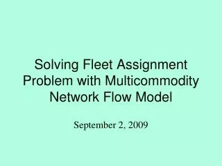
Multicommodity Network Flow [s11, s12,… s1K] cik, cost per unit at arc of commodity k [d11, d12,… d1K] S1 D1 cSD11, cSD12,… cSD1K uSD11, uSD12,… uSD1K cST11… cTD11… Transshipment Node sik, supply at node Si of commodity k dik, demand at node Di of commodity k uST11… uTD1…1 T1 Supply Nodes Demand Nodes Objective Function: cST21… cTD21… [s21, s22,… s2K] [d21, d22,… d2K] uST21… uTD21… S2 D2 cSD21… uSD21… uik, capacity at arcarc of commodity k
Multicommodity Network Flow • In multicommodity network flow problem, each arc has a finite capacity that applies to the sum of all commodities flowing over. • Also, each node must receive a particular amount of each type of commodity. • eg. A metal supplier ships aluminum bars, stainless steel rings, steel beams, etc. using a single limited capacity fleet of trucks. • In general form, the multicommodity network problem is defined as • Subject to: • For each commodity k and node t: • For each link i, j: Dik = demand for commodity k at node i, with negative values denoting supply; Cijk= cost per unit of shipping commodity k from node i to node j; Uij= capacity of the link from node i to node j; Xijk= amount of commodity k shipped from node i to node j.
MCN Flow Model – Fleet Assignment • Indices: • k, index for fleet types • v, index for nodes • i, index for arcs • h, index for airports • Input Parameters: • K, number of fleet types • V, set of all nodes • I, set of all arcs • IF, set of flight arcs • nk, number of available aircraft for fleet k • H, set of all airports • sh, the node associated with airport h and the beginning of the day • th, the node associated with airport h and the end of the day • cki, cost of assigning fleet k to flight arc I • Decision Variable: • xki, indicating whether fleet type k is assigned to arc i Decision Variable For the objective function: subject to Cost
Multicommodity Network Flow – Ex (2) F221 F105 F223 F259 F228 F230 F412 F238 GC2400 CHI 8:00 9:00 11:00 14:00 14:23 15:21 19:59 21:21 GC1100 GC1423 GC1521 GC1959 GC0800 GC0900 GC1400 F293 F766 F221 F228 F238 F223 F274 F230 GD2400 DEN 9:34 10:39 11:00 11:26 12:00 14:00 18:00 19:12 GD1100 GD0934 GD1039 GD1126 GD1200 GD1420 GD1800 F274 F105 F412 F293 F766 F259 GL2400 LAX 8:00 13:14 14:00 15:10 16:00 16:09 GL1400 GL1314 GL0800 GL1510 GL1600 • Diagonal lines (with the connection to its partner) constitute flight variables, Fxxx, where xxx represents flight number. • At each departure and arrival, including the end of the day (midnight), we suppose that there are decision variables of the numbers of aircraft on the ground, G(C,D, or L)hhmm,where hhmm represents time instance.
Multicommodity Network Flow – Ex (3) • Assumes that there are two types of aircraft , aircraft A and B, and that all profit contributions for each combination of aircraft and flight are known, we get • Thus, the C-plex code for the objective function of this example is: • For conservation of flow constraints, each instant of either an arrival or a departure constitutes a node, so: • (no. of aircraft on ground at this city at this instant) + (arrivals at this instant) • = (no. of departures from this city at this instant) + (no. of aircraft on the ground after this instant). maximize 105*F221A + 121*F221B + 109*F223A + 108*F223B + 110*F274A + 115*F274B + 130*F105A + 140*F105B + 106*F228A + 122*F228B + 112*F230A + 115*F230B + 132*F259A + 129*F259B + 115*F293A + 123*F293B + 133*F412A + 135*F412B + 108*F766A + 117*F766B + 116*F238A + 124*F238B;
Multi Commodity Network Flow – Ex (4) • The previous statement gives 22 constraints and 33 variables for one type of aircraft. However, the number of constraints and variables can be reduced if • a) Each arrival is delayed until the first departure after that arrival • b) Each departure is advanced (made earlier) to the most recent departure just after an arrival. GC2400 GC1400 GC2400 2 1 F221 F105 F223 F259 F228 F230 F412 F238 CHI 4 GD2400 8:00 9:00 11:00 14:00 14:23 15:21 19:59 21:21 GD1100 GD1800 3 F293 F766 F221 F228 F238 F223 F274 F230 5 GD2400 DEN 9:34 10:39 11:00 11:26 12:00 14:00 18:00 19:12 7 GL1600 GL2400 GL1400 GL2400 GL0800 F274 F105 F412 F293 F766 F259 6 9 8 LAX 8:00 13:14 14:00 15:10 16:00 16:09
Multi Commodity Network Flow – Ex (5) • The reduced flow conservation constraints can be described in C-plex as • T /*Conservation of flow constraints for type A aircraft*/ /*Chicago at 8am, sources - uses = 0*/ -F221A - F223A - F105A - F259A - GC1400A + GC2400A == 0; /*Chicago at midnight*/ F228A + F230A + F412A + F238A + GC1400A - GC2400A == 0; /*Denver at 11 AM*/ F221A + F223A - F228A - GD1100A + GD2400A == 0; /*Denver at high noon*/ F274A - F230A - F293A - F238A + GD1100A - GD1800A == 0; /*Denver at midnight*/ F766A - GD2400A + GD1800A == 0; /*LA at 8 AM*/ - F274A - GL0800A + GL2400A == 0; /*LA at 1400*/ F105A - F412A + GL0800A - GL1400A == 0; /*LA at 1600*/ F293A - F766A + GL1400A - GL1600A == 0; /*LA at midnight*/ F259A - GL2400A + GL1600A == 0; Must be repeated for type B aircraft
Multi Commodity Network Flow – Ex (6) • Then, in order to guarantee that each flight will be covered by at most one plane, we impose the following constraints: • which is converted to C-plex code as F221A + F221B <= 1; F223A + F223B <= 1; F274A + F274B <= 1; F105A + F105B <= 1; F228A + F228B <= 1; F230A + F230B <= 1; F259A + F259B <= 1; F293A + F293B <= 1; F412A + F412B <= 1; F766A + F766B <= 1; F238A + F238B <= 1;
Multi Commodity Network Flow – Ex (7) • If we set a limit on number of aircraft type B as 2 aircrafts, then the constraint • can be converted to C-plex code as • Finally, the 0-1 constraint on each flight arc can be carried out by declaring the flight decision variables as Boolean type: GC2400B + GD2400B + GL2400B <= 2; dvar boolean F221A; dvar boolean F221B; dvar boolean F223A; dvar boolean F223B; . . .
Multi Commodity Network Flow – Ex (8) • Running the C-plex code with ILOG, the solution is obtained as // solution (optimal) with objective 1325 F223A = 1; F274A = 1; F105A = 1; F230A = 1; F259A = 1; F412A = 1; F238A = 1; F221B = 1; F228B = 1; F293B = 1; F766B = 1; GC2400A = 3; GD1100A = 1; GL2400A = 1; GC2400B = 1; GD1100B = 1; GD2400B = 1;