DIVERSIFYING SELECTION AND FUNCTIONAL CONSTRAINT: ESTIMATING

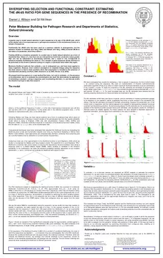
1. www.medawar.ox.ac.uk www.stats.ox.ac.uk/mathgen www.neisseria.org DIVERSIFYING SELECTION AND FUNCTIONAL CONSTRAINT: ESTIMATING THE dN/dS RATIO FOR GENE SEQUENCES IN THE PRESENCE OF RECOMBINATION Daniel J. Wilson and Gil McVean Peter Medawar Building for Pathogen Research and Departments of Statistics, Oxford University Overview A popular way to model natural selection in gene sequences is by way of the dN/dS ratio, which is the relative rate of non-synonymous to synonymous mutations in the evolutionary history of a sample of sequences. Traditionally the dN/dS ratio has been used as a summary statistic in phylogenetics, but the mutation models of Goldman and Yang (1994) and Nielsen and Yang (1998) promoted dN/dS to the status of a parameter, which they called ω. Treating dN/dS as a mutation parameter is a useful way to model natural selection as a form of mutational bias. Values of ω less than one are interpreted as functional constraint, values greater than one can be interpreted as diversifying selection, and ω equal to one corresponds to selective neutrality. Estimating the value of ω for a sample of gene sequences allows inference to be performed on the mode of selection acting on a region, or particular sites within that region. Maximum likelihood methods that estimate ω are in widespread use, and have been applied to many organisms. However, their common assumption of complete linkage along the sequence has been shown to lead to false positives when that assumption is violated by the presence of recombination (Schierup and Hein, 2000; Anisimova et al, 2003; Shriner et al, 2003). We present work-in-progress on a new method that aims, not only to estimate ω in the presence of recombination, but to co-estimate the recombination rate itself. We demonstrate its application in estimating a constant ω along a sequence, and in estimating site-wise ω’s, and discuss briefly the direction we hope to take this research. The model We adopted Nielsen and Yang’s (1998) model of mutation at the codon level, which defines the rate of mutation from codon i to codon j as where πj is the equilibrium frequency of codon j, λ is the rate of synonymous transversion per unit time (we use time units of PNe generations; P is the ploidy and Ne the effective population size), κis the transition to transversion ratio, and ω is the dN/dS ratio. Following Nielsen and Yang, we treat natural selection as a form of mutational bias which does not perturb the distribution of topology or branch lengths of the genealogical tree from the neutral probability model (which is owing to Kingman (1982) and, with recombination, Hudson (1983), Griffiths and Marjoram (1996)). Parameter estimation depends on evaluation of the likelihood function Pr(D|Θ), where D is the data, Θ = {λ, κ, ω, ρ}, and ρ is the recombination rate. Computational techniques have been developed that calculate the likelihood function by evaluating the likelihood given a tree and numerically integrate over trees, by Importance Sampling or Monte Carlo Markov Chain (MCMC). Such approaches are computationally intensive, extremely time consuming and are currently feasible only for estimation of a small number of parameters. Instead we make use of an approximation to the likelihood function (Li and Stephens, 2003) which we modify to incorporate the Nielsen and Yang mutation model. The algorithm for Li and Stephens’ “PAC” likelihood is extremely fast, and is based on reducing the dependency structure between trees along a sequence down to a Hidden Markov Model (HMM), where mutation is modelled in the emission probability. In our modification, we make the emission probability explicitly dependent on our mutation parameters λ, κ, and ω, so that we can evaluate the likelihood with respect to them. Figure 2 Sampling distributions for ML estimates of λ, κ, ω, ρ for 100 datasets simulated with ω = 0.25 (red histograms) and 100 datasets simulated with ω = 10 (yellow histograms). Each dataset consists of 20 sequences, length 300bp, under fixed λ = 1.0, κ = 6.0, ρ = 2.0 per codon. For λ, κ andρ, the sampling distributions are largely overlapping, but the ML estimates correctly distinguish between ω = 0.25 and ω = 10. However, for ω = 10 the ML estimates are considerably downwards biased. Estimates of λ appear to be upwardly biased. The means of the sampling distributions for λ and κ are somewhat elevated for ω = 10, suggesting that there is overlap in the information used to estimate λ, κ andω; this may explain the downwards bias in the ML estimate of ω. Constant ω We have investigated two models for estimating ω from a sample of sequences, the first of which treats ω as constant along the sequence. We used an implementation of Powell’s multi-dimensional optimization algorithm (Press et al, 2002) to obtain maximum likelihood estimates of all four parameters in the constant ω model. To study the properties of the ML estimates we simulated 20 sequences of length 300bp under fixed λ = 1.0, κ = 6.0, ρ = 2.0. One hundred simulations were performed with ω = 0.25 and another 100 with ω = 10. For each simulated data set, the ML estimates were obtained and the resulting sampling distributions for these estimates are illustrated in figure 2. The ML estimates exhibit bias (see figure 2 legend), and the estimates of mutation parameters appear to be sensitive to one another’s values, suggesting that there is some overlap in the information ML utilises. That the ML estimates are biased is perhaps unsurprising, however the parameters are of the correct order of magnitude, and the method appears to be capable of distinguishing between functional constraint and diversifying selection. As well as being biased, the ML estimates do not communicate the gradient of the likelihood surface around those point estimates, and asymptotic results for confidence intervals cannot be reliably applied. For these reasons we have adopted a Bayesian approach to parameter estimation, and we apply this to estimation in the case of variable ω. Figure 1 Example of a log likelihood surface with respect to ω and ρ, using our modification to the PAC likelihood. The data consisted of 50 simulated sequences of length 1000 codons generated under the following parameters: λ = 1.0, κ = 6.0, ω = 0.25, ρ = 2.0. The maximum likelihood estimates of ω and ρ are 0.17 and 1.5 respectively, or 0.25 and 1.5 when the true values of λ and κ are provided. The log likelihood surface is plotted for the true values of λ and κ. Figure 3 Posterior distributions for ω at each of ten sites in a simulated dataset. Green histograms: ω = 0.25. Red histograms: ω = 10. Variable ω To estimate ω in a site-wise manner, we employed an MCMC sampler to generate the posterior distribution of ω at each codon in a simulated dataset. We simulated a 10-codon sequence for n = 50, λ = 1.0, κ = 6.0, ρ = 2.0 and two values of ω. Sites 0-3, 8 and 9 were simulated under functional constraint (ω = 0.25, green histograms in figure 3) while sites 4-7 were simulated under diversifying selection (ω = 10, red histograms). To generate the site-wise posterior distributions of ω, all other parameters were held constant at their true values, and the MCMC sampler was run for 500,000 iterations. We chose an exponential prior on ω with mean 10 (shallow lines in figure 3). On first glance, there is no evidence that the posterior distributions of ω for sites under diversifying selection (red histograms) are higher than for sites under functional constraint (green histograms). However, when generating the data, we recorded the posterior distribution of ω given the true tree at each site, using the pruning algorithm (Felsenstein, 1981). This is illustrated by the other black lines in figure 3. The histograms for the posterior distributions, which use the approximate likelihood to integrate over trees, are fit the by the true posteriors remarkably well. This indicates two things. Firstly, the MCMC sampler and the likelihood are working very well, despite the approximate nature of the likelihood model. Secondly, even knowing the true genealogy cannot help us to distinguish between sites with high and low ω’s. For this simulated dataset, for example, it would be simply impossible to distinguish the codons under diversifying selection from the constrained sites, at least in a site-wise manner. Nevertheless, if contiguous codons share a common ω, we could apply a model in which the sequence is split into several sections, within which codons have the same ω. In a Bayesian framework, we can specify a prior on the number of splits in a given sequence, and using reversible-jump MCMC, we hope to be able to sample from the posterior number and positions of these splits. In this way we hope to improve on our site-wise approach by combining information from contiguous sites, enabling us to estimate ω along sequences that have experienced recombination. The PAC likelihood is based on expanding the likelihood function Pr(D|Θ) into a product of conditional likelihoods Pr(D1|Θ)Pr(D2|D1,Θ)…Pr(Dn|D1,…Dn-1,Θ). PAC approximates Pr(Dk+1|D1,…,Dk,Θ) using an HMM, in which the (k+1)th sequence is a mosaic of the first k sequences, which may be imperfect owing to mutation. At a given site, the HMM latent variable specifies which of the k other sequences the (k+1)th is a copy of. Along the sequence, recombination is modelled by switching the latent variable between the k other sequences. Thus, the (k+1)th sequence can be a copy of different sequences at different sites, but the structure of the HMM makes it likely that contiguous sites are copies from the same sequence. We use the same HMM for recombination along the sequence, but we modify the way that mutation is treated. In particular, we make explicit the idea of a time t to the common ancestor of the (k+1)th sequence and the sequence it copies from. We approximate the distribution of t as an exponential random variate with rate k. At each site, we take the probability (under the Nielsen and Yang model) of observing the codon at the (k+1)th sequence and the codon at the sequence that is copied, given the time t to their common ancestor, and integrate over t. This, the emission probability, is a function of λ, κ, and ω, so we can evaluate the likelihood with respect to these parameters. Figure 1 shows an example of the log-likelihood evaluated using this approximation, plotted against ω and ρ, with λ and κ fixed at their maximum likelihood (ML) point estimates. The data consisted of 20 simulated sequences, of length 300bp, generated with λ = 1.0, κ = 6.0, ω = 0.25, ρ = 2.0 per codon. In the expansion of the likelihood function Pr(D|Θ) into a product of conditional likelihoods, the order in which the sequences are labelled 1,…,n is irrelevant; they are exchangeable. But it the PAC likelihood, because the conditional likelihoods are only approximate, the ordering is relevant. Therefore, when we evaluate the likelihood function, we average over several orderings of the sequences, chosen at random. In the examples presented here, we average over ten orderings. The ten chosen orderings are preserved when evaluating the likelihood at different parameter values. Acknowledgments Thanks go to Stephen Leslie and Jonathan Marchini for help and advice, and to the BBSRC for funding. Cited References Anisimova et al (2003) Genetics164: 1229-1236 Felsenstein (1981) J Mol Evol17: 368-376 Goldman and Yang (1994) Mol Biol Evol11: 725-736 Griffiths and Marjoram (1996) J Comput Biol3: 479-502 Hudson (1983) Theor Popul Biol23: 183-201 Kingman (1982) J Appl Probab19A: 27-43 Li and Stephens (2003) Genetics165: 2213-2233 Nielsen and Yang (1998) Genetics148: 929-936 Press et al (2002) Numerical Recipes in C++. CUP Schierup and Hein (2000) Genetics156: 879-891 Shriner et al (2003) Genet Res81: 115-121