Statistical physics and finance
Statistical physics and finance. I. Kondor Collegium Budapest and Eötvös University Seminar talk at Morgan-Stanley Fixed Income Budapest, March 1, 2007. Coworkers. Sz. Pafka (ELTE; CIB Bank; Paycom, Santa Monica) G. Nagy ( Debrecen University; CIB Bank)


Statistical physics and finance
E N D
Presentation Transcript
Statistical physics and finance I. Kondor Collegium Budapest and Eötvös University Seminar talk at Morgan-Stanley Fixed Income Budapest, March 1, 2007
Coworkers • Sz. Pafka(ELTE; CIB Bank; Paycom, Santa Monica) • G. Nagy (Debrecen University; CIB Bank) • R. Karádi (Budapest University of Technology; Procter&Gamble) • N. Gulyás (ELTE; Budapest Bank; Lombard Leasing; ELTE; Collegium Budapest) • I. Varga-Haszonits István (ELTE; Morgan-Stanley) • G. Papp (ELTE) • A. Ciliberti (Roma and Science&Finance, Paris) • M. Mézard (Orsay)
Contents • Links between economics and physics • What can physics offer to finance that mathematics might not? • Three examples: random matrices, phase transitions and replicas
Early links • The physics-complex of classical economics • Maxwell • Bachelier
Physicists in finance • From the early nineties on financial institutions hire more and more physicists. • Some 30-35% of the invited speakers of risk managements conferences are ex-physicists. • Today finance is one of the standard fields of employment for physics graduates and PhD’s (EU document on the harmonization of the Bologna-type higher education curricula: Tuning Educational Structures in Europe: http://tuning.unideusto.org/tuningeu/ ).
Econophysics – is there such a thing? • The term was introduced by H. E. Stanley, it is not universally beloved, but wide-spread. • Do these two disciplines have anything to do with each other? • A trivial answer: we are dealing with stochastic processes in finance, and statistical physics is their main field of application. • But: the theory of stochastic processes in its pure form belongs to probability theory.
So the question is: Why do banks hire not only probabilists, applied mathematicians, computer scientists, statisticians, etc., but also physicists? • What is the special knowledge or skill, if any, that physicists can bring into finance? What can physics offer to finance? (Stanley at the Nikkei conference) • A common, albeit vague, answer: modeling skills, „creative” use of mathematics, knowledge of a wide spectrum of approximation and numerical methods, etc. may contribute to the market value of physicists.
A bit deeper: • Physics has got the farthest in the understanding of strongly interacting systems and collective phenomena. • Textbook-economics is, at best, on the conceptual level of mean-field theory even today (representative agent). • The building up of structures and new qualities from simple interactions, emergence, collective coordinates, averaging over microscopic degrees of freedom, etc. – these conceptual tools are not known in finance or economics at large (cf. Basel II).
Therefore I think that some knowledge ofquantum mechanics, many body problem, field theory, renormalisation, phase transitions, nonlinear and complex systems, etc., although neither necessary nor sufficient, may be useful (as a conceptual introduction or just as a source of metaphores) in the understanding of social phenomena, including the market.
In this talk I will illustrate the use of conceptual tools imported from physics on the following three examples: • Random matrices • Phase transitions and critical phenomena • Replica method
The concrete field of application will be the problem of portfolio selection • The basic question: How to distribute our wealth over the set of possible investment instruments so that to earn the highest return at the lowest risk? • Here I will focus my attention on the minimal risk portfolio, irrespective of the return.
The original formulation of the problem: The returns , i=1,2,…,N, are random variables drawn from a known (say, multivariate normal) distribution, with covariance matrix ( is the correlation matrix, the standard deviation of ). Find the weights , , for which the variance of the portfolio is minimal.
Unconstrained „short selling” We have not stipulated that the weights be positive, they can be of either sign, with an arbitrarily large absolute value. This is obviously unrealistic, for, among other things, liquidity reasons. Nevertheless, it is useful to consider the problem first in this idealised form (just as the finance text-books do), because then the optimal weights can be calculated analytically: If we ban short selling, the task becomes one in quadratic programming.
Infinite volume limit • Allowing unlimited short selling makes the domain of the optimization task infinite. This is not an innocent idealisation, because, as we will see, the solution vector can show huge fluctuations, and the restriction on the domain could bound these fluctuations . • Similarly to the theory of phase transitions, however, it is expedient to understand the essence of the phenomenon in the limit of infinite volume, and take into account the finite-volume effects only later.
Variants of the problem • When we use the standard deviation as a risk measure, we are assuming that the underlying process is normal, or has some similarly concentrated distribution. Typically, financial processes are not like this. • Alternative risk measures: mean absolute deviation (MAD), average loss above a high threshold (ES), maximal loss (ML), or, indeed, any homogeneous convex functional defined over the distribution of the losses.
Empirical covariance matrices • The covariance matrix has to be determined from measurements on the market. From the returns observed at time t we have the estimator: • The number of covariance matrix elements of a portfolio composed ofNinstruments isO(N²). In the time series of length T of N instruments we haveNTdata. In order to have a precise estimate, we should haveN <<T. Large portfolios can contain hundreds of instruments, while it is hardly meaningful to use data older than, say, 4 years, that is T~1000. Therefore the inequality N/T << 1almost never holds in reality. Thus our estimates will contain a lot of noise, and the estimation error will depend on the scaling variableN/T.
Information deficit • Thus the Markowitz problem suffers from the „curse of dimensions”, or from information deficit • The estimates will contain error and the resulting portfolios will be suboptimal • How serious is this effect? • How sensitive are the various risk measures to this kind of error? • How can we reduce the error?
Fighting the curse of dimensions • Economists have been struggling with this problem for ages. Since the root of the problem is lack of sufficient information, the remedy is to inject external info into the estimate. This means imposing some structure on σ. This introduces bias, but beneficial effect of noise reduction may compensate for this. • Examples: • single-index models (β’s) All these help to • multi-index models various degrees. • grouping by sectors Most studies are based • principal component analysis on empirical data • Bayesian shrinkage estimators, etc. • Random matrix theory
Origins of random matrix theory (RMT) • Wigner, Dyson 1950’s • Originally meant to describe (to a zeroth approximation) the spectral properties of heavy atomic nuclei - on the grounds that something that is sufficiently complex is almost random - fits into the picture of a complex system, as one with a large number of degrees of freedom, without symmetries, hence irreducible, quasi random. - markets, by the way, are considered stochastic for similar reasons
RMT • Later found applications in a wide range of problems, from quantum gravity through quantum chaos, mesoscopics, random systems, etc., etc. • Has developed into a rich field with a huge set of results for the spectral properties of various classes of random matrices • They can be thought of as a set of „central limit theorems” for matrices
Wigner semi-circle law • Mij symmetrical NxN matrix with i.i.d. elements (the distribution has zero mean and finite second moment) • k: eigenvalues of • The density of eigenvalues k (normed by N) goes to the Wigner semi-circle for N→∞ with prob. 1: , , otherwise
Remarks on the semi-circle law • Can be proved by the method of moments (as done originally by Wigner) or by the resolvent method (Marchenko and Pastur and countless others) • Holds also for slightly dependent or non-homogeneous entries • The convergence is fast (believed to be of ~1/N, but proved only at a lower rate), especially what concerns the support
Wishart matrices Generate very long time series for N iid random variables, with an arbitrary distribution of finite variance, and cut out samples of length T from these, as if making empirical observations. The „true” covariance matrix of these variables is the unit matrix, but if we try to reconstruct this from the simulated samples we will not recover the unit matrix for any finite T. Instead, we will have an „empirical” covariance matrix.
Correlation matrix of iid normal random variables The spectrum consists of a single, N-fold degenerate eigenvalue λ = 1 The noise lifts the degeneracy and makes a band out of the single eigenvalue. 1 0 C=
The corresponding „empirical” covariance matrix is the Wishart matrix If NandT→∞ such, that their ratio r =N/Tis fixed, < 1, then the spectrum of this empirical covariance matrix will be theWishart or Marchenko-Pastur spectrum (eigenvalue distribution): where
Remarks • The theorem also holds when the (average) sample covariance matrixis of finite rank • The assumption that the entries are identically distributed is not necessary • If T < N the distribution is the same with an extra point of mass 1 – T/N at the origin • If T = N the Marchenko-Pastur law is the squared Wigner semi-circle • The proof extends to slightly dependent and inhomogeneous entries • The convergence is fast, believed to be of~1/N , but proved only at a lower rate
N=1000 T/N=2
If the matrix elements are not centered but have, say, a common mean, one large eigenvalue breaks away, the rest stay in the random band Eigenvector components: just as in the Wigner case, the eigenvectors in the bulk are random, the one outside is „delocalized” (has nonzero entries everywhere) There is a lot of fluctuation, level crossing, random rotation of eigenvectors taking place in the random band The eigenvector belonging to the large eigenvalue (when there is one) is much more stable. The larger the eigenvalue, the moreso.
An intriguing observation • L.Laloux, P. Cizeau, J.-P. Bouchaud, M. Potters, PRL83 1467 (1999) and Risk12 No.3, 69 (1999) and V. Plerou, P. Gopikrishnan, B. Rosenow, L.A.N. Amaral, H.E. Stanley, PRL83 1471 (1999) noted that there is such a huge amount of noise in empirical covariance matrices that it may be enough to make them useless. • A paradox: Covariance matrices are in widespread use and banks still survive ?!
Laloux et al. 1999 The spectrum of the covariance matrix obtained from the time series of S&P 500 with N=406, T=1308, i.e. N/T= 0.31, compared with that of a completely random matrix (solid curve). Only about 6% of the eigenvalues lie beyond the random band.
Remarks on the paradox • The number of junk eigenvalues may not necessarily be a proper measure of the effect of noise: The small eigenvalues and their eigenvectors fluctuate a lot, indeed, but perhaps they have a relatively minor effect on the optimal portfolio, whereas the large eigenvalues and their eigenvectors are fairly stable. • The investigated portfolio was too large compared with the length of the time series (although it is hard to find a better ratio in practice). • Working with real, empirical data, it is hard to distinguish the effect of insufficient information from other parasitic effects, like nonstationarity (which is why we prefer to work with simulated data for the purposes of theoretical studies).
A filtering procedure suggested by RMT • The appearence of random matrices in the context of portfolio selection triggered a lot of activity, mainly among physicists. Laloux et al. and Plerou et al. proposed a filtering method based on random matrix theory (RMT) subsequently. This has been further developed and refined by many workers. • The proposed filtering consists basically in discarding as pure noise that part of the spectrum that falls below the upper edge of the random spectrum. Information is carried only by the eigenvalues and their eigenvectors above this edge. Optimization should be carried out by projecting onto the subspace of large eigenvalues, and replacing the small ones by a constant chosen so as to preserve the trace. This would then drastically reduce the effective dimensionality of the problem.
Interpretation of the large eigenvalues: The largest one is the „market”, the other big eigenvalues correspond to the main industrial sectors. • The method can be regarded as a systematic version of principal component analysis, with an objective criterion on the number of principal components. • In order to better understand this novel filtering method, I introduce a simple market model
Simple modell: market + sectors single - folddegenerate 1 - fold degenerate
The empirical covariance martix corresponding to this model consists of the Marchenko – Pastur spectrum, a large (Frobenius-Perron) eigenvalue (the whole market), and a number of medium-sized eigenvalues. If we resolve the equivalence of the sectors, with the appropriate tuning of the parameters we can mimic the spectrum observed on real markets (Noh model)
We have made extensive studies on the RMT-based filtering, and found that it performs consistently well compared with other, more conventional methods. • An additional advantage is that the method can be tuned according to the assumed structure of the market. • There are attempts to extract information from below the random band edge.
A measure of the effect of noise Assume we know the true covariance matrix and the noisy one . Then a natural, though not unique, measure of the impact of noise is where w*are the optimal weights corresponding to and , respectively.
The model-simulation approach For the purposes of our numerical calculations we chose various model covariance matrices and generated long simulated time series with them. Then we cut out segments of length T from these time series, as if observing them on the market, and tried to reconstruct the covariance matrices from them. We optimized a portfolio both with the „true” and with the „observed” covariance matrix and determined the measure .
Fluctuations over the samples • The relative error refers to a given sample, so it is a random variable that fluctuates from sample to sample. • Likewise, there are strong fluctuations in the weights of the optimal portfolio
The divergent error signals an algorithmic phase transition (I.K., Sz. Pafka, G. Nagy) • The rank of the covariance matrix is min{N,T} • In the limit N/T = 1 the lower band edge of eigenvalues goes to zero, around the lower edge there are many small eigenvalues – many soft modes. • N/T = 1 is the critical point of the problem • Upon approaching the critical point we find scaling laws, e.g. the expectation value of the portfolio error is: , while the standard deviation diverges as • For T<Nzero modes appear and the optimization becomes meaningless
Fluctuations of the weights:the distributionof the weights of a portfolio consisting of N=100 iid normal variables, in a given sample, for T=500
Sample to sample fluctuation of the weight of a given instrument, non-overlapping windows, N=100, T=500
Fluctuation of the weight of a given instrument, step by step moving average, N=100, T=500
After RMT filtering the error drops to an acceptable level and we can even penetrate the region T<N
Finite volume A ban on short selling, or any other constraint that renders the domain of optimization finite, or filtering will all supress the infinite fluctuations. However, the weights will keep wildly fluctuating as we approach N/T=1 and an increasing part of them will stick to the walls of the allowed region. These zero weights will belong to different instruments in different samples. If we are not sufficiently far away from the critical point, the solution of the Markowitz problem cannot serve as the basis of rational decision making.
Universality We have studied a number of different market models, different risk measures and different underlying processes (including fat tailed ones, and, with István Varga-Haszonits, also autoregressive, GARCH-like processes). The value of the critical point and the coefficients can change, but we have not yet found convincing evidence for any change in the critical exponents – we have not yet discovered the boundaries of the universality class.