Pixel-Based Processing
Pixel-Based Processing. ECE 847: Digital Image Processing. Stan Birchfield Clemson University. What is a digital image?. Accessing pixels in an image. Timing Test (640 x 480 image, get/set each pixel using 2.8 GHz P4). C / C++ Method 1: 1D array val = p[ y * width + x];

Pixel-Based Processing
E N D
Presentation Transcript
Pixel-Based Processing ECE 847:Digital Image Processing Stan Birchfield Clemson University
Accessing pixels in an image Timing Test(640 x 480 image, get/set each pixel using 2.8 GHz P4) C / C++ • Method 1: 1D arrayval = p[ y * width + x]; • Method 2: 2D arrayval = p[y][x]; • Method 3: pointersval = *p++; 6.6 ms 5.6 ms 0.5 ms (even faster with SIMD operations) Matlab • Method 1: 2D arrayval = im(y,x); • Method 2: parallelizeim = im + constant; 21.4 ms 2.5 ms
Histograms image histogram Throws away all spatial information!
Histogram equalization algorithm pdf Steps: • Compute normalized histogram (PDF)int hist[256] = 0…0float norm[256]for x, hist[ I(x) ]++for g in [0,255], norm[g] = hist[g] / npixels • Compute cumulative histogram (CDF)for g in [0,255], cum[g] = cum[g-1] + norm[g] • Transformfor x, I(x) = 255*cum[ I(x) ] equal area cdf equal spacing new gray level old gray level
Thresholding Valley separates light from dark How to find it?
A simple thresholding algorithm Repeat until convergence: T ½ (m1 + m2) [Gonzalez and Woods, p. 599]
Otsu’s method • Threshold t splits image into two groups • Calculate within-group variance of each group • Search over all t to minimize total within-group variance; recursive relations make search efficient percentage of pixelsin first group variance of pixelsin first group
Local Entropy Thresholding(LET) • Compute co-occurrence matrix • Threshold s divides matrix into four quadrants • Pick s that maximizesHBB(s)+HFF(s) • Uses spatial information
Otsu vs. LET image histogram Otsu LET
Adaptive thresholding background image histogram from Gonzalez and Woods, p. 597
Double thresholding (hysteresis) graylevel threshold too high: misses part of object object 2 object 1 threshold too low: captures noise noise pixel • Algorithm: • Threshold with high value • Threshold with low value, retaining only thepixels that are contiguous with existing ones
Double thresholding example image low threshold retains some background combined high threshold removes some foreground
Neighbors 4-neighborsN4 8-neighbors N8 diagonal neighbors ND
Adjacency • 4-adjacency: • 8-adjacency: • m-adjacency: p q p q or and Example: 4 8 m
Adjacency Use different connectedness for foreground and background to avoid inconsistency foreground: D8 background: D4 dumbbell
Connectivity, Regions and Boundaries • path from p to q is sequence of adjacent pixels • p and q are connected in subset S if path exists between them containing only pixels in S • connected component of p is set of pixels in S that are connected to p • S is a region if it is a connected set • boundary of S is the set of pixel in S that have one or more neighbors not in S
Morphological operations • morphology – form and structure • We will deal only with binary images • Set theory review • union • intersection • difference • complement • Two fundamental operations:Dilation and Erosion
Dilation • A and B are sets in Z2 • image A • structuring element B • Algorithm: • Flip B (but often symmetric) • Move B around • Anywhere they intersect, turn center pixel on • Looks like nonlinear convolution
Dilation (cont.) Let B be 3x3 with all 1s.for y for x if ( in(x-1, y) || in(x-1, y-1) || in(x-1, y+1) ... || in(x+1, y+1)) out(x, y) = 1 else out(x, y) = 0 B A
Erosion • Algorithm: • Move B around • If there is not complete overlap, turn center pixel off • Duality between dilation and erosion • This is why B is flipped in dilation
Erosion (cont.) Let B be 3x3 with all 1s.for y for x if ( in(x-1, y) && in(x-1, y-1) && in(x-1, y+1) ... && in(x+1, y+1)) out(x, y) = 1 else out(x, y) = 0 B A
Closing and Opening • Dilation fills gaps. Erosion removes noise • Combine them: • First dilate, then erode (closing) • First erode, then dilate (opening) • Closing/opening retain object size • Repeated applications do nothing • Duality between closing and opening
Morphology Example open then close erode dilate close open thresholded difference
Accessing out-of-bounds pixels • If kernel is near boundary of image, some pixels of kernel will be out of bounds (OOB) • What to do? • Do not use OOB pixels (change kernel size near boundary) • Do not compute output for pixels near boundary • Extend image function: • zero pad – OOB pixels have value of zero • replicate – OOB pixels have value of closest pixel • reflect – pixel values are extended by mirror reflection at border • wrap – pixel values are extended by repeating • extrapolate – pixel values are extended by extrapolating function near boundary • No solution is best • Problem also occurs with convolution
Floodfill • Fill a region with a new color • Start with a seed point • All pixels are colored if they have the same color as the seed and are connected to the seed via pixels that have the same color as the seed
Floodfill Repeated applications of dilation can fill a region image A structuring element B complement Ac ... but terribly inefficient
Floodfill Efficient implementation uses a stack called the frontier. Function image = Floodfill(seed_point, image, new_color) old_color = image(seed_point) frontier.Push(seed_point) image(seed_point) = newcolor while (NOT frontier.IsEmpty()) q = frontier.Pop(); for each neighbor r of q, if image(r) == old_color, frontier.Push(r) image(r) = new_color return image frontier:
Connected components • Recall that connected component of p is set of pixels in S that are connected to p • Can solve the problem by repeated applications of Floodfill – assigning a new label to each new region • More efficient implementation involves two passes through the image (union-find)
Connected component labeling scan left-to-right, top-to-bottom U L P I(P) == I(U) ? 4-neighbor algorithm: I(P) == I(L) ? 4-neighbor mask: 8-neighbor mask:
Connected components:first pass 0 0 0 0 0 1 1 1 1 0 2 2 2 2 0 3 3 3 2 4 3 5 5 2 4 image components equivalence table
Connected components:traverse table 0 0 0 0 0 1 1 1 1 0 2 2 2 2 0 3 3 3 2 4 3 5 5 2 4 image components equivalence table
Connected components:second pass 0 0 0 0 0 1 1 1 1 0 0 0 0 0 0 3 3 3 0 4 0 0 0 0 4 image components equivalence table
Connected components Function labels = ConnectedComponents(image) // first pass for y=0 to height-1, for x=0 to width-1, pix = image(x,y) if pix == image(x-1,y) && pix == image(x,y-1) labels(x,y) = labels(x,y-1) SetEquivalence(labels(x-1,y), labels(x,y-1)) else if pix == image(x-1,y) labels(x,y) = labels(x-1,y) else if pix == image(x,y-1) labels(x,y) = labels(x,y-1) else labels(x,y) = next_label++ // second pass for y=0 to height-1, for x=0 to width-1, labels(x,y) = GetEquivalentLabel( labels(x,y) )
Connected components Function SetEquivalence(a, b) aa = GetEquivalentLabel(a) bb = GetEquivalentLabel(b) if aa > bb equiv[aa] = bb else if aa < bb equiv[bb] = aa Function b = GetEquivalentLabel(a) if a == equiv[a] return a else equiv[a] = GetEquivalentLabel(equiv[a]) return equiv[a]
Connected components quantized image components
Perimeter • Perimeter of binary region: • Dilate, then subtract • Erode, then subtract • (Which is better?) • This only gives the pixels as binary image • To get ordered list of contiguous pixels, use Wall Follow algorithm
Wall following Algorithm: • If pixel to the left is ON, Turn left and move forward • Else if pixel in front is OFF, Turn right • Else move forward - This traverses clockwise, using 4-connectedness (other versions are possible) - Can be used to compute perimeter
Distance functions • D is a distance function (metric) if • Common distance functions: shape of each?
Length along path Freeman formula c = 0 (overestimates) Pythagorean theorem c = 1(underestimates) Kimura’s method c = ½(good compromise) isothetic (solid) diagonal (hollow) path (not necessarily straight line) 3 methods compared
Chamfering • How to approximate “correct” distance (Euclidean)? • Along a path, • Let m be number of isothetic moves (horizontal or vertical) • Let n be number of diagonal moves • Define chamfer distance between p and q as dab = min {am+bn} over all possible paths • Chamfer distance is metric if a, b > 0 • If b > 2a, then diagonal moves are ignored • Special cases: • a=1, b=infinity (Manhattan) • a=1, b=1 (chessboard) • a=1, b=sqrt(2) (another reasonable choice) • a=1, b=1.351 (best approximation to Euclidean) • a=3, b=4 (best integer approximation, scaled by factor of 3) [G. Borgefors, Distance transformations in digital images, CVGIP, 1986]
Chamfering (cont.) • Chamfering is process of computing distance to each foreground pixel • Two-pass algorithm • Traverse top-to-bottom, left-to-right • Traverse bottom-to-top, right-to-left In each case, compute minimum distance F: B: F: B: 4-connectivity 8-connectivity
Chamfering (cont.) Function labels = Chamfer(image) // first pass for y=0 to height-1, for x=0 to width-1, d(x,y) = image(x,y) ? 0 : min(infinity, 1+d(x-1,y), 1+d(x,y-1)) // second pass for y=height-1 to 0 step -1, for x=width-1 to 0 step -1, d(x,y) = image(x,y) ? 0 : min(d(x,y), 1+d(x+1,y), 1+d(x,y+1)) • Algorithm (for D4 using Manhattan distance):
Uses of chamfering • Find center of biggest part of shape • Shape matching (Gavrila) • Useful for watershed thresholding centroid largest chamfer value
Integral image • Integral image is analogous to summed area table (SAT) in graphics • To compute, S(x,y) = I(x,y) - S(x-1,y-1) + S(x-1,y) + S(x,y-1) • To use, V(l,t,r,b) = S(l,t) + S(r,b) - S(l,b) - S(r,t)Returns sum of values inside rectangle • Note: Sum of values in any rectangle can be computed in constant time!
Skeletons • Point on skeleton is equidistant to >= 2 boundary points(without crossing) • Or, equivalently, • where wavefronts (grassfires) meet (shock graph) • centers of maximal balls • Blum’s Medial Axis Transform (MAT) • Skeleton is highly sensitive to noise
Skeletonization by thinning • First compute MAT • Then delete points such that • do not remove endpoints • do not break connectivity • do not excessively erode region