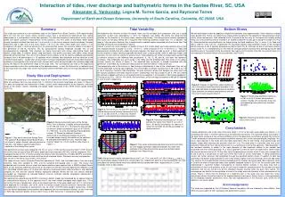
Interaction of tides, river discharge and bathymetric forms in the Santee River, SC, USA Alexander E. Yankovsky , Legna

1. Interaction of tides, river discharge and bathymetric forms in the Santee River, SC, USA Alexander E. Yankovsky, Legna M. Torres Garcia, and Raymond Torres Department of Earth and Ocean Sciences, University of South Carolina, Columbia, SC 29208, USA Summary This study was carried out in the freshwater reach of the Santee River (South Carolina, USA) approximately 55±4 km from the river mouth, where transition occurs from a two-directional tidally-driven flow regime downstream to a unidirectional riverine flow upstream. The data set comprises a bathymetric survey, current profile and bottom pressure measurements at two locations, and time series of discharge. Water depth reveals threefold variations from less than 2 m to over 5 m in the form of adjacent shoals and deeps. Complex bathymetry and a high ratio of the wave height (~0.5 m) to the mean water depth over shoals (~2 m) exceeding 0.25 result in nonlinear dynamics of the observed tidal waves. The nonlinear effects are evident in the generation of the M4 harmonic. The M4 along-channel velocity amplitude exceeds 40% of the corresponding M2 amplitude. Tidal velocities are highly asymmetric with strong, short-lasting floods and weaker, longer ebbs. In addition, bottom drag coefficients also exhibit asymmetry with higher values being observed during the flood. The ratio of the subtidal riverine velocity to the M2 velocity amplitude dramatically increases from 0.48 downstream to 1.15 upstream which indicates tidal dissipation and the transition to the river-dominated regime. Combination of asymmetric nonlinear tides/bottom drag with strong tidal dissipation produces a convergence of the maximal shear stresses which occur during the ebb at the upstream edge and during the flood at the downstream edge of the study area. This convergence can lead to the trapping of coarse sediments and to the maintenance of the observed shoals. In fact, the thickness of a sediment layer in the study area was larger than further downstream where intermittent areas of the exposed bedrock were found. Study Site and Deployment This study was carried out in the freshwater reach of the Santee River (South Carolina, USA) approximately 55±4 km upstream from the river mouth (Fig. 1). Details of the channel morphology are shown in Figure 2. Our data set comprises two bathymetric surveys, current profile measurements at two locations, and time series of the stream velocity, discharge and gauge height measured at the USGS stream gauge station 02171700 . Two bathymetric surveys were conducted, the first, on June 4, 2008, and the second on April 7, 2009. During the 2008 survey we used a Ross 875 sonar, depth data were acquired at 200 kHz, and we sampled at 10Hz, averaging the data at 1Hz. The echo sounder and receiver were connected to a Trimble G8 GPS, and linked by cellular modem-internet to the state real-time virtual reference station. Positional accuracy and precision was ±0.02m in the lateral, and ±0.03m in the vertical. The second survey used a Sysquest Strata Box operating at 10kHz, and it provided returns from two major reflectors. Data were sampled at 10Hz, and the sampling and logging were in sync. The survey was conducted over the same channel reach and vessel positions were acquired with a WAAS-enabled Garmin GPS, at ±3m accuracy. Depth accuracies are on the order of 0.02m but manually digitizing the reflectors using CTI SonarWeb software gave a 0.1m pixel size. Based on field observations of bed and banks, and sediment sampling we infer that the second reflector represents bedrock. Where the first and second reflectors converged we interpreted as exposed bedrock channel, whereas reflector divergence represented a thickening alluvial deposit. We deployed two upward-looking ADCPs mounted on bottom tripods and separated by an approximately 6-km along-channel distance. At the upstream site R, the mean (tidally-averaged) water depth was 1.78 m during the first day of deployment, while at the downstream site S the water depth was 3.27 m. Instruments were deployed for a fortnight, July 16-30, 2008, in relatively straight reaches of channel. Hereinafter, time of the deployment is measured as starting from July 16, 2008, 12:00 PM (local daylight saving time). At both sites the Nortek Aquadopp current profilers were deployed, but their configuration differed: at site S we used a 1-MHz high-resolution profiler, while at site R it was a 2-MHz instrument in standard configuration. Tidal Variability We determine the direction of both the record mean and the principal axis component; they are in good agreement at both sites (discrepancy is within 5-7 degrees) (see Table). We define the along-channel direction as the direction of the record mean, positive downstream. The along-channel velocity component time series are low-pass filtered with a Gaussian filter retaining oscillations longer than 1 hr. In addition, we apply a 1-day low-pass Gaussian filter to demonstrate a subtidal regime associated with the riverine flow. The resulting time series are presented in Figure 3. Overall, currents are more energetic at location R due to the smaller depth and cross-sectional area at this site. Subtidal velocity at location S is only ~ 0.04 m s-1, while at location R it is ~0.16-0.18 m s-1. Tides are predominantly semidiurnal with visible asymmetry between the flood and ebb currents: a flood (upstream) current reaches a higher velocity magnitude but peaks over a shorter period, while an ebb lasts longer and maintains its near-maximal velocity for several hours. Tidal properties are further characterized by performing a harmonic analysis of the following tidal constituents: K1, M2, S2, M4 and M6 (the latter two represent overtides). Tidal amplitudes are summarized in the Table and the predicted tidal time series of the along-channel velocity are shown in Figure 4. The observed tidal asymmetry is indeed associated with the generation of overtides, M4 in particular (likely due to the nonlinear effects in tidal dynamics). The comparative role of the riverine vs. tidal forcing is illustrated by a ratio of the record-mean flow (set by riverine discharge) to the M2 tidal amplitude. This ratio exhibits a dramatic increase from 0.48 at site S to 1.15 at site R implying a significant tidal dissipation. We also estimate a phase shift between the water level and the velocity oscillations (the latter lead the former). Interestingly, time lag is larger at site S (140 min) where the channel is deeper but there is a strong bathymetric convergence in the direction of tidal wave propagation. Time lag at site R is ~105 min. For the M2 tidal constituent, these time lags correspond to 68 and 51 degrees at sites S and R, respectively. Table. Along-channel velocity characteristics at site S, z=1.17 m, and site R, z=1.05 m. Here αmean and αprax are the directions [deg] of record mean and principal axis, respectively, positive is counterclockwise from east; and σu are the velocity record mean and subtidal velocity standard deviation, respectively [m s-1]; tidal amplitude refers to tidal velocity. Bottom Stress We estimate bottom stress by applying a logarithmic boundary layer approximation, which requires a steady state, parallel flow. Hence, we select those velocity profile samples for the logarithmic fitting procedure which satisfy these requirements. Data collected at site R proved to be too noisy for the logarithmic velocity profile fitting. Our strict screening criteria resulted in an excellent alignment of data points along the straight line (Fig. 6). Estimated bottom drag coefficients are higher during the flood conditions (Fig. 7): mean Cd for flood and ebb is 1.88×10-2 and 1.06×10-2, respectively. An asymmetric bottom drag coefficient results in the strongest bottom stresses at site S typically developing during the flood (Fig. 8). Although we did not estimate a bottom stress at site R, it is straightforward to infer that the strongest bottom stresses there develop during the ebb conditions due to the predominantly downstream flow regime at this location (Fig. 3b). As a result, there is a convergence of maximum bottom stresses between sites R and S. Conclusions Complex bathymetry and a high ratio of the wave height (~0.5 m) to the mean water depth over shoals (~2 m) exceeding 0.25 result in nonlinear dynamics of the observed tidal waves. The nonlinear effects are evident in the asymmetric structure of free surface oscillations and in the generation of overtides, primarily M4 harmonic. The M4 amplitude of along-channel velocity oscillations exceeds 40% of the corresponding M2 amplitude. As a result, tidal velocities in the study area are highly asymmetric (Fig. 3) with strong, short-lasting floods and weaker, longer ebbs retaining near-constant values for ~6 hr. The study area is a transition zone from a two-directional tidally-driven flow regime downstream to a unidirectional riverine flow upstream. Tidal dissipation in the upstream direction is evident in the rapid decrease of tidal amplitude relative to the subtidal flow associated with the riverine discharge. As a result, upstream currents at site R are weak and in several cases the reversal did not occur at all. On the other hand, the downstream currents at site R are much stronger than at site S due to a combination of tidal and riverine flow fields of similar magnitudes. A strong downstream current can further enhance tidal dissipation through the quadratic bottom stress. In addition to tidal flow asymmetry, the bottom drag coefficient at site S also exhibits higher values for the flood versus the ebb stage. This leads to the strongest bottom stresses developing at this location during the flood. Mean absolute values of Cd are one order of magnitude higher than typically accepted values of O(10-3) for the coastal ocean often implemented in numerical models. Convergence of maximal bottom stresses in the study area (that is, downstream at site R and upstream at site S) can have an important consequence for the transport of coarse sediments that can be moved only by the strongest stresses exerted under the given flow regime. This convergence can lead to the accumulation of sand in the study area and ultimately to the maintenance of the shoals. Figure 2 shows that the thickness of a sediment layer in the study area was larger than further downstream where intermittent areas of the exposed bedrock were found. Hence, there is a strong possibility for the feedback between bathymetric forms and tidal hydrodynamics in the transition zone, which we will address in our future studies. Acknowledgements This study was supported by the US National Science Foundation. We are indebted to Jason Walker, Scott White and Lew Lapine for their assistance with bathymetric surveys. Figure 6. Samples of logarithmic velocity profiles at site S that satisfy screening criteria described in the text, flood (left panel) and ebb (right panel) conditions. Black asterisks are velocity measurements and red lines are the least-squares linear fit. Figure 7. Bottom drag coefficient relative to z=0.62 m at site S versus along-channel velocity. Triangle with vertical bar shows the corresponding mean plus/minus standard deviation. Figure 3. Time series of 1-hr and 24-hr low-pass filtered along-channel velocity measured at site S, z=1.17 (a) and at site R, z=1.05 m (b). Positive/ negative is the downstream/upstream direction. Figure 8. Along-channel bottom shear stress versus time at site S. Figure 4. Harmonic tidal analysis of 1-hr low-passed time series from Figure 3: (a) sum of the K1, M2 and S2 constituents; (b) same as in (a) but the overtides M4 and M6 are added; (c) residual currents. Figure 2. Along-channel bathymetry of the Santee River, 0 km is arbitrary. A) depth to the channel bed on 6/17/08 with Q=72 m3/s. B) shows the channel bed as alluvium (black) and bedrock (gray) on 4/7/09 with Q = 906 m3/s. C) is the line representing the bedrock surface. D) Shows the sediment thickness determined as the difference between B) and C). Inverted triangles identify the location of the upstream R and downstream S ADCP sites. Note the large channel “deeps” at ~2.5 km and 8 km (also shown in Figure 1 ). Figure 1. (Top) aerial view of the Santee River. The upstream R and downstream S ADCP sites are shown in yellow. (Bottom) channel planform at high flow. The bridge is approximately 55 km upstream of the Santee River mouth. Figure 5. Time series of band-passed water level at R and S sites (a); time-lagged correlation coefficient between the water level oscillations from Figure 5a and the along-channel tidal velocity prediction from Figure 4b (b).