
14-B 餘數的計算
14-B 餘數的計算. (1) x (mod M ) 的值,必定為 0 ~ M −1 之間 (2) a + b (mod M ) = { a (mod M ) + b (mod M )} (mod M ) 例: 78 + 123 (mod 5) = 3 + 3 (mod 5) = 1 (Proof): If a = a 1 M + a 2 and b = b 1 M + b 2 , then a + b = ( a 1 + b 1 ) M + a 2 + b 2

14-B 餘數的計算
E N D
Presentation Transcript
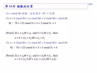
14-B 餘數的計算 (1) x (mod M) 的值,必定為 0 ~ M−1 之間 (2) a + b (mod M) = {a (mod M) + b (mod M)} (mod M) 例: 78 + 123 (mod 5) = 3 + 3 (mod 5) = 1 (Proof): If a = a1M + a2 and b = b1M + b2 , then a + b = (a1 + b1)M + a2 + b2 (3) ab (mod M) = {a (mod M) b (mod M)} (mod M) 例: 78 123 (mod 5) = 3 3 (mod 5) = 4 (Proof): If a = a1M + a2 and b = b1M + b2 , then ab = (a1 b1M + a1b2 + a2b1)M + a2b2
在 Number Theory 當中 只有 M2個可能的加法, M2個可能的乘法 可事先將加法和乘法的結果存在記憶體當中 需要時再 “LUT”
14-C Properties of Number Theoretic Transforms P.1) Orthogonality Principle proof : P.2) The NTT and INTT are exact inverse proof :
P.3) Symmetry f(n) = f(Nn) F(k) = F(Nk) f(n) = f(Nn) F(k) = F(Nk) NTT NTT P.4) INNT from NTT Algorithm for calculating the INNT from the NTT (1) F(-k) : time reverse F0, F1, F2, …, FN-1F0, FN-1, …, F2, F1 (2) NTT[ F(k) ] (3) 乘上 time reverse
P.5) Shift Theorem P.6) Circular Convolution (the same as that of the DFT) P.7) Parseval’s Theorem
P.8) Linearity P.9) Reflection If then
If N (transform length) is a power of 2, then the radix-2 FFT butterfly algorithm can be used for efficient calculation for NTT. Decimation-in-time NTT Decimation-in-frequency NTT The prime factor algorithm can also be applied for NTTs. 14-D Efficient FFT-Like Structures for Calculating NTTs
One N-point NTT Two (N/2)-point NTTs plus twiddle factors where
Bit reversal Original sequence f(n) = (1, 2, 0, 0) N = 4, M = 5 Permutation (1, 0, 2, 0) After the 1st stage (1, 1, 2, 2) After the 2nd stage F(k) = (3, 0, 4, 2) α0=1 α0=1 α2=4 α1=2 α2=4 α0 α2 α3=3
Inverse NTTby Forward NTT : 1) 1/N 2) Time reversal 3) permutation 4) After first stage 5) After 2nd stage α0=1 α0=1 Permutation α2=4 α1=2 Time reversal α2=4 α0 α2 α3=3
14-E Convolution by NTT 假設x[n] = 0 for n < 0 and n K,h[n] = 0 for n < 0 and n H 要計算x[n] h[n] = z[n] 且 z[n] 的值可能的範圍是 0 z[n] < A (more general, A1 z[n] < A1 + T) (1) 選擇 M(the prime number for the modulus operator), 滿足 (a) M is a prime number, (b) M max(H+K, A) (2) 選擇 N (NTT 的點數), 滿足 (a) N is a factor of M1, (b) N H+K 1 (3) 添0: x1[n] = x[n] for n = 0, 1, ……, K1, x1[n] = 0 for n = K, K +1, ……., N1 h1[n] = h[n] for n = 0, 1, ……, H1, h1[n] = 0 for n = H, H +1, ……., N 1
(4)X1[m] = NTTN,M{x1[n]}, H1[m] = NTTN,M {h1[n]} NTTN,M指N-point 的DFT (mod M) (5)Z1[m] = X1[m]H1[m], z1[n] = INTTN,M {Z1[m]}, (6)z[n] = z1[n] for n = 0, 1, …., H+K 1 (移去 n = H+K, H+K+1, …… N1 的點) (More general, if we have estimated the range of z[n] should be A1 z[n] < A1 + T, then z[n] = ((z1[n] − A1))M + A1
適用於(1) x[n],h[n]皆為整數 (2) Max(z[n]) − min(z[n])< M的情形。 Consider the convolution of (1, 2, 3, 0) * (1, 2, 3, 4) Choose M = 17, N = 8,結果為:
Max(z[n]) − min(z[n]) 的估測方法 假設 x1 x[n] x2, 則 (Proof): where h1[m] = h[m] when h[m] > 0 , h1[m] = 0 otherwise h2[m] = h[m] when h[m] < 0 , h2[m] = 0 otherwise
Fermat Number : P = 0, 1, 2, 3, 4, 5, ….. M = 3, 5, 17, 257, 65537, … Mersenne Number : M = 2p − 1 P = 1, 2, 3, 5, 7, 13, 17, 19 M = 1, 3, 7, 31, 127, 8191, ….. If M = 2p − 1 is a prime number, p must be a prime number. However, if p is a prime number, M = 2p − 1 may not be a prime number. 14-F Special Numbers
The modulus operations for Mersenne and Fermat prime numbers are very easy for implementation. 2k 1 Example: 25 mod 7 a = −1 100
The integer field ZM can be extended to complex integer field If the following equation does not have a sol. in ZM 無解 This means (-1) does not have a square root When M = 4k +1, there is a solution for x2 = −1 (mod M). When M = 4k +3, there is no solution for x2 = −1 (mod M). For example, when M = 13, 82 = −1 (mod 13). 21 = 2, 22 = 4, 23 = 8, 24 = 3, 25 = 6, 26 = 12 = −1, 27 = 11, 28 = 9, 29 = 5, 210 = 10, 211 = 7, 212 = 1 When M = 11, there is no solution for x2 = −1 (mod M). 14-GComplex Number Theoretic Transform (CNT)
If there is no solution for x2 = −1 (mod M), we can define an imaginary number i such that i2 = −1 (mod M) Then, “i” will play a similar role over finite field ZM such that plays over the complex field.
14-HApplications of the NTT NTT 適合作 convolution 但是有不少的限制 新的應用: encryption (密碼學) CDMA
References: (1) R. C. Agavard and C. S. Burrus, “Number theoretic transforms to implement fast digital convolution,” Proc. IEEE, vol. 63, no. 4, pp. 550- 560, Apr. 1975. (2) T. S. Reed & T. K Truoay, ”The use of finite field to compute convolution,” IEEE Trans. Info. Theory, vol. IT-21, pp.208-213, March 1975 (3) E.Vegh and L. M. Leibowitz, “Fast complex convolution in finite rings,” IEEE Trans ASSP, vol. 24, no. 4, pp. 343-344, Aug. 1976. (4) J. H. McClellan and C. M. Rader, Number Theory in Digital Signal Processing, Prentice-Hall, New Jersey, 1979. (5) 華羅庚, “數論導引”, 凡異出版社, 1997。
XIV. Orthogonal Transform and Multiplexing 14-A Orthogonal and Dual Orthogonal Any M N discrete linear transform can be expressed as the matrix form: Y = A X inner product
Orthogonal: when k h • orthogonal transforms 的例子: • discrete Fourier transform • discrete cosine, sine, Hartley transforms • Walsh Transform, Haar Transform • discrete Legendre transform • discrete orthogonal polynomial transforms • Hahn, Meixner, Krawtchouk, Charlier
為什麼在信號處理上,我們經常用 orthogonal transform? Orthogonal transform 最大的好處何在?
If partial terms are used for reconstruction for orthogonal case, perfect reconstruction: partial reconstruction: K < N reconstruction error of partial reconstruction 由於 一定是正的,可以保證 K越大, reconstruction error 越小
For non-orthogonal case, perfect reconstruction: partial reconstruction: B = A−1 K < N reconstruction error of partial reconstruction 由於 不一定是正的, 無法保證 K越大, reconstruction error 越小
14-B Frequency and Time Division Multiplexing 傳統 Digital Modulation and Multiplexing:使用 Fourier transform Frequency-Division Multiplexing Xn = 0 or 1 Xn can also be set to be −1 or 1 When (1) t [0, T] (2) fn = n/T it becomes the orthogonal frequency-division multiplexing (OFDM).
Furthermore, if the time-axis is also sampled t = mT/N, m = 0, 1, 2, ….., N−1 then the OFDM is equivalent to the transform matrix of the inverse discrete Fourier transform (IDFT), which is one of the discrete orthogonal transform. Modulation:
Modulation: Demodulation: Example: N = 8 Xn = [1, 0, 1, 1, 0, 0, 1, 1] (n = 0 ~ 7)
Time-Division Multiplexing (also a discrete orthogonal transform)
思考: 既然 time-division multiplexing 那麼簡單 那為什麼要使用 frequency-division multiplexing 和 orthogonal frequency-division multiplexing (OFDM)?
14-C Code Division Multiple Access (CDMA) 除了 frequency-division multiplexing 和 time-division multiplexing,是否還有其他 multiplexing 的方式? 使用其他的 orthogonal transforms即 code division multiple access (CDMA) CDMA is an important topic in spread spectrum communication 參考資料 [1] M. A. Abu-Rgheff, Introduction to CDMA Wireless Communications, Academic, London, 2007 [2] 邱國書, 陳立民譯, “CDMA 展頻通訊原理”, 五南, 台北, 2002.
CDMA 最常使用的 orthogonal transform 為 Walsh transform channel 1 channel 2 channel 3 channel 4 channel 5 channel 6 channel 7 channel 8
當有兩組人在同一個房間裡交談 (A 和B交談), (C 和D交談) , • 如何才能夠彼此不互相干擾? • 不同時間 • (2) 不同聲調 • (3) 不同語言
CDMA 分為: (1) Orthogonal Type (2) Pseudorandom Sequence Type Orthogonal Type 的例子:兩組資料[1, 0, 1] [1, 1, 0] (1) 將 0 變為 −1 [1, −1, 1] [1, 1, −1] (2) 1, −1, 1 modulated by [1, 1, 1, 1, 1, 1, 1, 1] (channel 1) [1, 1, 1, 1, 1, 1, 1, 1, -1, -1, -1, -1, -1, -1, -1, -1, 1, 1, 1, 1, 1, 1, 1, 1] 1, 1, −1 modulated by [1, 1, 1, 1, -1, -1, -1, -1] (channel 2) [1, 1, 1, 1, -1, -1, -1, -1, 1, 1, 1, 1, -1, -1, -1, -1, -1, -1, -1, -1, 1, 1, 1, 1] (3) 相合 [2, 2, 2, 2, 0, 0, 0, 0, 0, 0, 0, 0, -2, -2, -2, -2, 0, 0, 0, 0, 2, 2, 2, 2]
demodulation [2, 2, 2, 2, 0, 0, 0, 0, 0, 0, 0, 0, -2, -2, -2, -2, 0, 0, 0, 0, 2, 2, 2, 2] [1, 1, 1, 1, 1, 1, 1, 1] [1, 1, 1, 1, 1, 1, 1,1] [1, 1, 1, 1, 1, 1, 1, 1] 內積 = 8
注意: (1) 使用 N-point Walsh transform 時,總共可以有N個 channels (2) 除了 Walsh transform 以外,其他的 orthogonal transform 也可以使用 (3) 使用 Walsh transform 的好處
Orthogonal Transform 共通的問題: 需要同步 synchronization R1 = [ 1, 1, 1, 1, 1, 1, 1, 1] R2 = [ 1, 1, 1, 1, 1, 1, 1, 1] R5 = [ 1, 1, 1, 1, 1, 1, 1, 1] R8 = [ 1, 1, 1, 1, 1, 1, 1, 1] 但是某些basis, 就算不同步也近似 orthogonal <R1[n], R1[n]> = 8, <R1[n], Rk[n]> = 0 if k 1 <R1[n], Rk[n1]> = 2 or 0 if k 1.
Pseudorandom Sequence Type 不為 orthogonal,capacity 較少 但是不需要同步(asynchronous) Pseudorandom Sequence 之間的correlation b1p(t+ 1) + b2p(t + 2) recovered: (若 C(0) = 1, C(21) 0) 1, 2不必一致 C() -axis
CDMA 的優點: (1) 運算量相對於 frequency division multiplexing 減少很多 (2) 可以減少noise 及interference的影響 (3) 可以應用在保密和安全傳輸上 (4) 就算只接收部分的信號,也有可能把原來的信號recover 回來 (5) 相鄰的區域的干擾問題可以減少
相鄰的區域,使用差距最大的「語言」,則干擾最少相鄰的區域,使用差距最大的「語言」,則干擾最少 B 區 A 區 假設 A 區使用的 orthogonal basis 為 k[n], k = 0, 1, 2, …, N−1 B 區使用的 orthogonal basis 為 h[n], h = 0, 1, 2, …, N−1 設法使 為最小 k = 0, 1, 2, …, N−1, h = 0, 1, 2, …, N−1
附錄十四 3-D Accelerometer 的簡介 3-D Accelerometer: 三軸加速器,或稱作加速規 許多儀器(甚至包括智慧型手機) 都有配置三軸加速器 可以用來判別一個人的姿勢和動作 應用: 動作辨別 (遊戲機) 運動 (訓練,計步器) 醫療復健,如 Parkinson 患者照顧,傷患復原情形 其他 (如動物的動作,機器的運轉情形的偵測)
z-axis y-axis x-axis 根據 x, y, z三個軸的加速度的變化,來判斷姿勢和動作 平放且靜止時, z-axis 的加速度為 –g = – 9.8
若加速規傾斜, z-axis 的加速度將不再是 – 9.8, 沿著 x和 y軸的加速度不再是 0
例子:若將加速規放在腳上……………. 走路時,沿著其中一個軸的加速度變化
期末的勉勵 人生難免會有挫折,最重要的是,我們面對挫折的態度是什麼 想一想,就連舉世聞名的 Fourier transform,也是 1812 年投稿,中間被退稿很多次,直到 1822年才被接受、刊登,比較起來,我們已經算是很幸運了 長遠的願景可以美麗,短期的目標要務實
祝各位同學暑假愉快! 各位同學在研究上或工作上,有任何和digital signal processing 或time frequency analysis 方面的問題,歡迎找我來一起討論。