Download
1 / 70
700 likes | 855 Vues
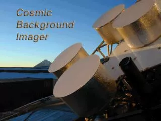
The Cosmic Background Imager (CBI), located in the Andes mountains of Chile, is a cutting-edge facility designed to study the Cosmic Microwave Background (CMB). A collaborative effort involving major institutions such as Caltech, NRAO, and more, the CBI utilizes advanced technology including 13.90-cm Cassegrain antennas and HEMT amplifiers to capture detailed images of the CMB. Through its observations, the CBI aims to unravel the early universe's thermal history and the anisotropies imprinted during the recombination era, shedding light on cosmic evolution and fundamental cosmological parameters.

E N D
The Cosmic Background Imager Steven T. Myers National Radio Astronomy Observatory Socorro, NM
The Cosmic Background Imager • A collaboration between • Caltech (A.C.S. Readhead PI) • NRAO • CITA • Universidad de Chile • University of Chicago • With participants also from • U.C. Berkeley, U. Alberta, ESO, IAP-Paris, NASA-MSFC, Universidad de Concepción • Funded by • National Science Foundation, the California Institute of Technology, Maxine and Ronald Linde, Cecil and Sally Drinkward, Barbara and Stanley Rawn Jr., the Kavli Institute, and the Canadian Institute for Advanced Research
The Instrument • 13 90-cm Cassegrain antennas • 78 baselines • 6-meter platform • Baselines 1m – 5.51m • 10 1 GHz channels 26-36 GHz • HEMT amplifiers (NRAO) • Cryogenic 6K, Tsys 20 K • Single polarization (R or L) • Polarizers from U. Chicago • Analog correlators • 780 complex correlators • Field-of-view 44 arcmin • Image noise 4 mJy/bm 900s • Resolution 4.5 – 10 arcmin
Other Interferometers: DASI, VSA • DASI @ South Pole • VSA @ Tenerife
CBI Operations • Observing in Chile since Nov 1999 • NSF proposal 1994, funding in 1995 • Assembled and tested at Caltech in 1998 • Shipped to Chile in August 1999 • Continued NSF funding in 2002, to end of 2004 • Telescope at high site in Andes • 16000 ft (~5000 m) • Located on Science Preserve, co-located with ALMA • Now also ATSE (Japan) and APEX (Germany), others • Controlled on-site, oxygenated quarters in containers • Data reduction and archiving at “low” site • San Pedro de Atacama • 1 ½ hour driving time to site
The Cosmic Microwave Background • Discovered 1965 (Penzias & Wilson) • 2.7 K blackbody • Isotropic • Relic of hot “big bang” • 3 mK dipole (Doppler) • COBE 1992 • Blackbody 2.725 K • Anisotropies 10-5
Thermal History of the Universe Courtesy Wayne Hu – http://background.uchicago.edu
CMB Anisotropies • Primary Anisotropies • Imprinted on surface of “last scattering” • “recombination” of hydrogen z~1100 • Primordial (power-law?) spectrum of potential fluctuations • Collapse of dark matter potential wells inside horizon • Photons coupled to baryons >> acoustic oscillations! • Electron scattering density & velocity • Velocity produces quadrupole >> polarization! • Transfer function maps P(k) >> Cl • Depends on cosmological parameters >> predictive! • Gaussian fluctuations + isotropy • Angular power spectrum contains all information • Secondary Anisotropies • Due to processes after recombination
Power Spectrum of the CMB Courtesy Wayne Hu – http://background.uchicago.edu
Dependence on Geometry Courtesy Wayne Hu – http://background.uchicago.edu
Dependence on Baryon content Courtesy Wayne Hu – http://background.uchicago.edu
Effects of Damping Courtesy Wayne Hu – http://background.uchicago.edu
Secondary Anisotropies Courtesy Wayne Hu – http://background.uchicago.edu
Gravitational Secondaries • Due to CMB photons passing through potential fluctuations (spatial and temporal) • Includes: • Early ISW (decay, matter-radiation transition at last scattering) • Late ISW (decay, in open or lambda model) • Rees-Sciama (growth, non-linear structures) • Tensors (gravity waves, ‘nuff said) • Lensing (spatial distortions) Courtesy Wayne Hu – http://background.uchicago.edu
Scattering Secondaries • Due to variations in: • Density • Linear = Vishniac effect • Clusters = thermal Sunyaev-Zeldovich effect • Velocity (Doppler) • Clusters = kinetic SZE • Ionization fraction • Coherent reionization suppression • “Patchy” reionization
2ndary SZE Anisotropies • Spectral distortion of CMB • Dominated by massive halos (galaxy clusters) • Low-z clusters: ~ 20’-30’ • z=1: ~1’ expected dominant signal in CMB on small angular scales • Amplitude highly sensitive to s8 A. Cooray (astro-ph/0203048) P. Zhang, U. Pen, & B. Wang (astro-ph/0201375)
Seven Pillars of the CMB (of inflationary adiabatic fluctuations) • Large Scale Anisotropies • Acoustic Peaks/Dips • Damping Tail • Gaussianity • Secondary Anisotropies • Polarization • Gravity Waves Minimal Inflationary parameter set Quintessence Tensor fluc. Broken Scale Invariance
Images of the CMB WMAP Satellite BOOMERANG ACBAR
After WMAP… • Power spectrum • measured to l < 1000 • Primary CMB • First 3 peaks Courtesy Wayne Hu – http://background.uchicago.edu
…and Planck • Power spectrum • measured to l < 1000 • Primary CMB • First 6 peaks Courtesy Wayne Hu – http://background.uchicago.edu
Interferometers • Spatial coherence of radiation pattern contains information about source structure • Correlations along wavefronts • Equivalent to masking parts of a telescope aperture • Sparse arrays = unfilled aperture • Resolution at cost of surface brightness sensitivity • Correlate pairs of antennas • “visibility” = correlated fraction of total signal • Fourier transform relationship with sky brightness • Van Cittert – Zernicke theorem
The Fourier Relationship • The aperture (antenna) size smears out the coherence function response • Like a double-slit experiment with widening slits • Interference plus diffraction pattern • Lose ability to localize wavefront direction = field-of-view • Small apertures = wide field • An interferometer “visibility” in the sky and Fourier planes:
The uv plane and l space • The sky can be uniquely described by spherical harmonics • CMB power spectra are described by multipole l ( the angular scale in the spherical harmonic transform) • For small (sub-radian) scales the spherical harmonics can be approximated by Fourier modes • The conjugate variables are (u,v) as in radio interferometry • The uv radius is given by l / 2p • The projected length of the interferometer baseline gives the angular scale • Multipole l = 2pB / l • An interferometer naturally measures the transform of the sky intensity in l space
CMB peaks smaller than this ! Interferometry of the CMB • An interferometer “visibility” in the sky and Fourier planes: • The primary beam and aperture are related by: CBI:
Power Spectrum and Likelihood • Statistics of CMB (Gaussian) described by power spectrum: Construct covariance matrices and perform maximum Likelihood calculation: Break into bandpowers
CBI Beam and uv coverage • 78 baselines and 10 frequency channels = 780 instantaneous visibilities • Frequency channels give radial spread in uv plane • Pointing platform rotatable to fill in uv coverage • Parallactic angle rotation gives azimuthal spread • Beam nearly circularly symmetric • Baselines locked to platform in pointing direction • Baselines always perpendicular to source direction • Delay lines not needed • Very low fringe rates (susceptible to cross-talk and ground)
Calibration and Foreground Removal • Calibration scale ~5% • Jupiter from OVRO 1.5m (Mason et al. 1999) • Agrees with BIMA (Welch) and WMAP • Ground emission removal • Strong on short baselines, depends on orientation • Differencing between lead/trail field pairs (8m in RA=2deg) • Use scanning for 2002-2003 polarization observations • Foreground radio sources • Predominant on long baselines • Located in NVSS at 1.4 GHz, VLA 8.4 GHz • Measured at 30 GHz with OVRO 40m • Projected out in power spectrum analysis
Power Spectrum Estimation • Method described in Paper IV (Myers et al. 2003) • Large datasets • > 105 visibilities in 6 x 7 field mosaic • ~ 103 independent • Gridded “estimators” in uv plane • fast! • Not lossless, but information loss insignificant • Construct covariance matrices for gridded points • Maximum likelihood using BJK method • Output bandpowers • Wiener filtered images constructed from estimators
Tests with mock data • The CBI pipeline has been extensively tested using mock data • Use real data files for template • Replace visibilties with simulated signal and noise • Run end-to-end through pipeline • Run many trials to build up statistics
Wiener filtered images • Covariance matrices can be applied as Wiener filter to gridded estimators • Estimators can be Fourier transformed back into filtered images • Filters CX can be tailored to pick out specific components • e.g. point sources, CMB, SZE • Just need to know the shape of the power spectrum
Example – Mock deep field Noise removed Raw CMB Sources
CBI 2000 Results • Observations • 3 Deep Fields (8h, 14h, 20h) • 3 Mosaics (14h, 20h, 02h) • Fields on celestial equator (Dec center –2d30’) • Published in series of 5 papers (ApJ July 2003) • Mason et al. (deep fields) • Pearson et al. (mosaics) • Myers et al. (power spectrum method) • Sievers et al. (cosmological parameters) • Bond et al. (high-l anomaly and SZ) pending
CBI Deep Fields 2000 • Deep Field Observations: • 3 fields totaling 4 deg^2 • Fields at d~0 a=8h, 14h, 20h • ~115 nights of observing • Data redundancy strong tests for systematics
CBI 2000 Mosaic Power Spectrum • Mosaic Field Observations • 3 fields totaling 40 deg^2 • Fields at d~0 a=2h, 14h, 20h • ~125 nights of observing • ~ 600,000 uv points covariance matrix 5000 x 5000
Cosmological Parameters wk-h: 0.45 < h < 0.9, t > 10 Gyr HST-h: h = 0.71 ± 0.076 LSS: constraints on s8 and G from 2dF, SDSS, etc. SN: constraints from Type 1a SNae
SZE Angular Power Spectrum [Bond et al. 2002] • Smooth Particle Hydrodynamics (5123) [Wadsley et al. 2002] • Moving Mesh Hydrodynamics (5123) [Pen 1998] • 143 Mpc 8=1.0 • 200 Mpc 8=1.0 • 200 Mpc 8=0.9 • 400 Mpc 8=0.9 Dawson et al. 2002
Constraints on SZ “density” • Combine CBI & BIMA (Dawson et al.) 30 GHz with ACBAR 150 GHz (Goldstein et al.) • Non-Gaussian scatter for SZE • increased sample variance (factor ~3)) • Uncertainty in primary spectrum • due to various parameters, marginalize • Explained in Goldstein et al. (astro-ph/0212517) • Use updated BIMA (Carlo Contaldi) Courtesy Carlo Contaldi (CITA)
New : Calibration from WMAP Jupiter • Old uncertainty: 5% • 2.7% high vs. WMAP Jupiter • New uncertainty: 1.3% • Ultimate goal: 0.5%