Blind quantifiers
Episode 10. Blind quantifiers. Unistructurality The blind universal and existential quantifiers DeMorgan’s laws for blind quantifiers The hierarchy of quantifiers How blind quantification affects game trees. 0. 10.1. Unistructurality.

Blind quantifiers
E N D
Presentation Transcript
Episode 10 Blind quantifiers • Unistructurality • The blind universal and existential quantifiers • DeMorgan’s laws for blind quantifiers • The hierarchy of quantifiers • How blind quantification affects game trees 0
10.1 Unistructurality A game A is said to be unistructural iff, for any valuations e1 and e2, we have Lre1[A]=Lre2[A]. Intuitively, unistructural games are games all instances of which have the same structure. All of the examples of games that we have seen so far are unistructural, and so are all naturally emerging games. Also, all of our game operations preserve the unistructural property of games. Hence, if you wish, it is safe to assume that “game” always means “unistructural game”. For the sake of generality, however, we do not officially impose this unnecessary restriction on games. Our definition (next slide) of the blind quantifiersx (universal) and x (existential), however, assumes that the game A(x) to which they are applied satisfies the weaker condition of x-unistructurality. We say that a game A(x) is x-unistructural iff, for any valuation e and any two constants c and d, Lre[A(c)]=Lre[A(d)]. Intuitively, this means that the structure of any given instance of A does not depend on the value of x (but may depend on the values of some other variables). Of course, every unistructural game is also x-unistructural for any variable x.
10.2 Formal definitions of the blind quantifiers Definition 10.1. Let A(x)be an x-unistructural game. (a) The gamexA(x)is defined by: (b) The gamexA(x) is defined by: • LrexA(x)= LreA(x). • WnexA(x) = ⊤ iff, for all constants c, WneA(c) = ⊤. • LrexA(x)= LreA(x). • WnexA(x) = ⊥ iff, for all constants c, WneA(c) = ⊥. Intuitively, playing xA(x) or xA(x) means just playing A(x) “blindly”, without knowing the value of x. In xA(x), Machine wins iff the play it generates is successful for every possible value of x, while in xA(x) being successful for just one value is sufficient. When applied to elementary games, the blind quantifiers, just like the parallel quantifiers, act exactly as the quantifiers of classical logic.
10.3 DeMorgan’s laws for blind quantifiers From the definition one can see a perfect symmetry between and , ⊤and⊥. Therefore, just as for the choice and parallel quantifiers, DeMorgan’s laws hold: xA= xA xA= xA xA= xA xA= xA
10.4 x versus ⊓x Unlike xA(x) which is a game on infinitely many boards, both ⊓xA(x)and xA(x) are one-board games. Yet, they are very different from each other. To see this difference, compare the problems ⊓x(Even(x)⊔Even(x)) x(Even(x)⊔Even(x)) and Depth= 2 (Environment selects a number m, to which Machine replies by 0 or 1) Depth= 1 (only Machine has a move, 0 or 1) Winnable? Of course. Evenness is a decidable problem. Winnable? No. Machine cannot select a ⊔-disjunct that would be true for all values of x.
10.5 The hierarchy of quantifiers Easiest to win xA(x) xA(x) incomparable ⊔xA(x) ⊓xA(x) Hardest to win xA(x) xA(x) incomparable
10.6 How blind quantification affects game trees Suppose A is a unistructural game. To turn the game tree for A into a game tree for xA, just add the prefix “x” to each node of it. Similarly for xA. Even(x)⊔Odd(x) x (Even(x)⊔Odd(x)) ⊥ x ⊥ 0 1 0 1 Even(x) Odd(x) x Even(x) x Odd(x)
10.6 How blind quantification affects game trees Suppose A is a unistructural game. To turn the game tree for A into a game tree for xA, just add the prefix “x” to each node of it. Similarly for xA. Even(x)⊔Odd(x) x (Even(x)⊔Odd(x)) ⊥⊔⊥ ⊥ x ⊥ 0 1 0 1 Even(x) Odd(x) x Even(x) ⊥ x Odd(x) ⊥
10.7 x(Even(x)⊔Odd(x) ⊓y(Even(x+y)⊔Odd(x+y))) A computable -problem This problem is computable. The idea of a winning strategy is that, for any given y, in order to tell whether x+y is even or odd, it is not really necessary to know the value of x. Rather, just knowing whether x is even or odd is sufficient. And such knowledge can be obtained from the antecedent. In other words, for any known y and unknown x, the problem of telling whether x+y is even or odd is reducible to the problem of telling whether x is even or odd. Specifically, of both x and y are even or both are odd, then x+y is even; otherwise x+y is odd. Below is the evolution sequence induced by a run where Machine used a winning strategy. Game Move x(Even(x)⊔Odd(x) ⊓y(Even(x+y)⊔Odd(x+y))) 1.7 x(Even(x)⊔Odd(x) Even(x+7)⊔Odd(x+7)) 0.0 x(Even(x) Even(x+7)⊔Odd(x+7)) 1.1 x(Even(x) Odd(x+7)) The play hits ⊤, and thus Machine wins.
10.8 Exercise Do the following problems appear to be (always) computable? x(P(x)⊔P(x)) No x(P(x)P(x)) Yes x(P(x)P(x)P(x)) Yes x(P(x)P(x)P(x)) No xP(x)⊓xP(x) Yes ⊓xP(x) xP(x) No ⊓xP(x) xP(x) Yes x(P(x)Q(x)) (xP(x)xQ(x)) Yes ⊓x(P(x)Q(x)) (⊓xP(x)⊓xQ(x)) No ⊓xP(x)⊓xQ(x) ⊓x(P(x)Q(x)) Yes