Download

1 / 63
640 likes | 806 Vues
Debt-Equity Decision-Making with Wealth Transfer. Professor Robert M. Hull Clarence W. King Endowed Chair in Finance School of Business Washburn University 1700 SW College Avenue Topeka, Kansas 66621 (Phone: 785 393 5630) Email: rob.hull@washburn.edu

E N D
Debt-Equity Decision-Making with Wealth Transfer Professor Robert M. Hull Clarence W. King Endowed Chair in Finance School of Business Washburn University 1700 SW College Avenue Topeka, Kansas 66621 (Phone: 7853935630) Email: rob.hull@washburn.edu Tuesday, November 12, 2013; 12:30pm; HC 104
1. Introduction • With the inception of modern corporate finance over fifty years ago, there has been abundant empirical and theoretical research on the tax, bankruptcy, and agency impact from capital structure changes. • Yet there is a shortage of instructional exercises with practical formulas to illustrate these impacts. • This paper fills this void by concentrating on the agency impact stemming from wealth transfers between security owners. • The capital structure research question addressed in this paper is: “To what extent do wealth transfer effects between security holders influence security values when a levered firm undergoes a capital structure change?” • The instructional tool used to answer this question is the Capital Structure Model (CSM) pioneered by Hull (2007, 2010, 2012). • Since a major goal is to focus on an agency influence of leverage changes, we draw heavily from the recent CSM research of Hull (2012) that addresses wealth redistributions between equity and debt owners who share a principal-agent relation.
1. Introduction(continued) • Why use the CSM? The many bankruptcy and agency effects that can be involved in achieving an optimal GL are impractical to measure. • The CSM research makes the measurement task more manageable through its development of GL equations that require managers to only estimate tax, borrowing, and growth rates. • Incorporating a wealth transfer through a shift in risk among owners adds to the measurement task in that one must now estimate the extent that risk shifting lowers one security’s discount rate at the expense of an increase in another security’s discount rate. • While estimating rates required to use the CSM is a daunting task, it is one that financial managers should embrace if its leads to making proper debt-equity decisions.
1. Introduction(continued) • This paper builds on two prior CSM instructional exercises. • First, we extend the exercise of Hull (2008) that compared gain from leverage (GL) results using three perpetuity GLequations. These equations come from models supplied by (i) Modigliani and Miller (1963), referred to as MM, (ii) Miller (1977), and (iii) Hull (2007). • Second, we build on the Hull (2011) exercise that incorporates a growth situation tied to the plowback-payout choice. This exercise demonstrates the dangers of too much debt for growth firms.
1. Introduction (continued) • We maintain continuity with the latter two exercises by utilizing the same question and answer methodology and (where applicable) by using similar values for variables to compute GL. However, the scope of this paper's exercise is uniquely different in many ways. • First, unlike prior pedagogical perpetuity GL research, our starting point focuses on a levered firm as opposed to an unlevered firm. • Second, we have an incremental approach when computing GL. This approach is needed to handle a levered firm undergoing a series of debt-for-equity increments. • Third, we do what prior CSM instructional papers have not been able to do: separate equity’s GLversus debt’s GL. By doing this, equity’s GL is revealed to be different. • Fourth, we consider the principal-agent relationship that involves wealth redistribution among security holders. The overall gain to leverage can be shown to be different with a wealth transfer.
1. Introduction (continued) • The rest of this paper is as follows. • Section 2 gives the impetus, framework, learning outcomes and assessment process. • Section 3 reviews capital structure models concentrating on perpetuity GLequations. • Section 4 contains our instructional exercise. • Section 5 provides final remarks.
2. Impetus, framework and outcomes for learning exercise 2.1.Impetus • Prior studies (Leland, 1998; Graham and Harvey, 2001) suggest that capital structure is not taught at the level of other corporate finance topics. • One reason is because the “traditional” GL equations are not as creditable as those for capital budgeting or costs of capital. • The “non-traditional” CSM GL equations attempt to overcome the creditability problem. • The most basic CSM equations by Hull (2007) adopted the MM (1963) and Miller (1977) perpetuity approach for an unlevered growth firm. Subsequent CSM equations by Hull (2010, 2012) has continued this perpetuity format. • While MM describe the positive relation between debt and security borrowing rates, the MM and Miller GL equations do not demonstrate how changes in these rates lead to an optimal leverage choice. In contrast, the CSM equations show how changes in these rates cause an optimum. • In their recent review of the capital structure research, Graham and Leary (2011) suggest that researchers have studied the wrong models, examined incorrect issues, improperly measured key variables, and failed to furnish insight on firm behavior. • This indicates that new innovative capital structure research such as offered by the CSM should be explored. • The CSM claims to provide creditable equations capable of measuring tax, agency and bankruptcy effects stemming from leverage changes.
2. Impetus, framework and outcomes for learning exercise 2.1.Impetus (continued) • The impetus for this paper is two-fold. • First, there is the judgment by experts against the state of modern capital structure research its failure to provide teaching tools. • Second, there is the potential offered by the CSM research that supplies a system of equations capable of capturing leverage-related effects consistent with firm behavior. In particular, the recent CSM research by Hull (2012) develops GL equations to demonstrate the agency impact when wealth is transferred among security holders. • Given these wealth transfer equations, we have the necessary mathematical format to extend the Hull (2008, 2011) instructional exercises to incorporate wealth transfers stemming from principal-agent conflicts between debtholders and equityholders.
2. Impetus, framework and outcomes for learning exercise 2.2.Framework for incorporating wealth transfers • The nongrowth perpetuity GL research (MM, 1963; Miller, 1977; Hull, 2007) imparts no analysis of the roles of growth or wealth transfers. • To overcome the growth problem, Hull (2010) broadened the CSM framework by integrating the plowback-payout choice with the debt-equity choice. • Hull derives a critical point in order to estimate the minimum growth rate the firm must achieve to add value. The critical point is where the plowback ratio equals the cost of raising funds. He argues that the critical point could be as high as the effective corporate tax rate due to double taxation when using internal funds. • Hull formulates other new breakthrough concepts including the equilibrating unlevered and levered growth rates. He uses these two growth rates to get growth-adjusted discount rates needed to derive GL equations with growth. • Most recently, Hull (2012) derives GL equations showing how a wealth transfer (linked to a shift in risk) impacts firm value. These latter equations add a 3rd component to the tax-agency and bankruptcy components identified by Hull (2007). This 3rd component captures an agency effect represented by the wealth transfer between debt and equity owners.
2. Impetus, framework and outcomes for learning exercise 2.2. Framework for incorporating wealth transfers(continued) • The theoretical development by Hull (2012) provides the tool to extend the Hull (2008, 2011) pedagogical exercises so that educators now have a framework for teaching capital structure decision-making that will be applicable to leveraged firms undergoing incremental leverage changes that generate wealth transfers. • Using wealth transfer equations, teachers can potentially integrate a number of related corporate finance topics. These topics include: • Shift in risk among security holders as considered by Jensen and Meckling (1976) and Masulis (1980) • Asset substitution as encompassed in Jensen and Meckling (1976) and Leland (1998) • Underinvestment as discussed by Myers (1977) and Gay and Nam (1998) • The relation between an optimal leverage ratio and valuation effects as examined by Leland (1998) and Hull (1999)
2. Impetus, framework and outcomes for learning exercise 2.3.Learning outcomes and assessment • By partaking in this paper’s exercise, advanced business students with a strong background in corporate finance should comprehend the complexities of capital structure decision-making including agency complications. • The following learning outcomes should occur. • First, students should learn how to compute GLequations. • Second, students should gain experience in comparing GLequations based on the different assumptions under which they are derived (nongrowth versus growth or unlevered situation versus levered situation). • Third, students should learn the role of wealth transfers when making the debt-to-equity choice.
2. Impetus, framework and outcomes for learning exercise 2.3.Learning outcomes and assessment (continued) • GLexercises fall within learning goals related to quantitative reasoning and within the learning outcomes related to learning financial decision-making. • The outcome assessment process should include identification of measures to assess learning, analysis of the information given by the measures, and action to improve student performance. • Instructors should seek to answer questions such as “How will students learn desired outcomes?” and “How can instructors be sure students have learned outcomes at some minimal level?” • By using this paper’s exercise, instructors can assess whether students have mastered and achieved the learning outcomes at an acceptable level.
3. Gain from Leverage Research 3.1.General Research • Capital structure research (MM, 1958; Jensen and Meckling, 1976; Harris and Raviv, 1991; Mello and Parsons 1992; Myers, 2001; Strebulaev, 2007; Berk, Stanton, and Zechner, 2010; Korteweg, 2010)is rich and encompasses many features. • This paper focuses on one feature: the perpetuity gain from leverage (GL). This GL feature originates with MM (1963) and Miller (1977) and has been most recently continued by Hull (2007, 2010, 2012). • The next two subsections review the GL research focusing on the equations used in this paper.
3. Gain from Leverage Research 3.2. MM and Miller equations for GL • For a firm issuing perpetual debt to retire equity, MM (1963)present the gain from leverage (GL) as GL = TCD(1) where TC is the effective corporate tax rate and D = I/rF with I as the perpetual cash flow and rFas the riskless cost of debt. • Equation (1) disregards personal taxes, growth, agency effects and bankruptcy costs. • It also does not consider a levered situation thereby ignoring a wealth transfer involving outstanding debt. • Miller (1977) extends (1) by considering personal taxes to get GL = (1 − α)D(2) where α = (1TE)(1TC)/(1TD) with TEand TDas the personal tax rates on equity and debt income, respectively, and now D = (1TC)I/rDwith rDas the cost of debt. • Miller believes α ≈ 1 for any firm because personal and corporate taxes offset one another so that an optimal capital structure does not exist because GL is trivial for all debt choices • A trivial GLis consistent with Miller’s belief that leverage-related costs are inconsequential.
3. Gain from Leverage Research 3.2. MM and Miller equations for GL(continued) • Theoretically, most researchers disagree with Miller and favor optimal capital structure models. • Earlier theorists (Baxter, 1967; Kraus and Litzenberger, 1973; Jensen and Meckling, 1976), argue that GL is optimized when a further issuance of debt no longer makes incremental benefits outweigh incremental costs. • More recent theorists (Hennessy and Whited, 2005; Leary and Roberts, 2005; Korteweg, 2010) continue to advance this optimal notion. • Empirically, most researchers find that the leverage-related costs are substantial but there is not perfect agreement (Warner, 1977; Altman, 1984; Kayhan and Titman, 2007). • There are a few researchers who offer specific numbers concerning GL. Graham (2000), Korteweg (2010), and Van Binsbergen, Graham, and Yang (2010) collectively suggest that GL can be as much as 10% of firm value indicating that there is an optimal debt-equity mix where firms attain maximum positive leverage effects.
3. Gain from Leverage Research 3.3. CSM Nongrowth and Growth Equations for GL • Like MM and Miller, the early CSM research by Hull (2007) focused on an unlevered nongrowth firm. Given a nongrowth scenario where there is a plowback ratio of zero, Hull shows GL(nongrowth) = (3) where rU and rL are the costs of unlevered and levered equity, and EU(or VU) is the unlevered equity value for a nongrowth firm referred to as VU(nongrowth). • VU(nongrowth) equals whereC = (1–PBR)(CFBT) with PBRas the before-tax plowback ratio and CFBT as the perpetual before-tax cash flow generated by operating assets. For nongrowth, PBR = 0 and C = CFBT. • A positive GL in (3) can result even without a tax effect where α = 1. • This positive effect can be attributed to designing security types that reduce agency costs.
3. Gain from Leverage Research 3.3. CSM Nongrowth and Growth Equations for GL(continued) • Hull (2010) extends (3) by incorporating growth. • This leads to discounting equity cash flows by a growth-adjusted discount rate (analogous to the discounting in the constant growth DVM). • By incorporating growth, Hull shows GL(growth) = D EU(4) where rUgis the growth-adjusted discount rate on unlevered equity given as rUg= rUgUwith gUas the unlevered equity growth rate; rLgis the growth-adjusted discount rate on levered equity given as rLg =rLgL with gLas the levered equity growth rate; and,EU(or VU) is the unlevered equity value for a firm with growth and is referred to as VU(growth). • VU(growth) equals whereC = (1–PBR)(CFBT) with C < CFBTbecause PBR > 0.
3. Gain from Leverage Research 3.4. CSM Wealth Transfer Equations for GL • In practice, firms that issue debt are typically levered. They can approach a target leverage ratios over time by issuing incremental amounts of debt. When they stray from their target ratios, they issue securities as levered firms. • Thus, the prior GLequations can be criticized for focusing on an unlevered situation with only one debt-for-equity transaction made from among possible choices. • To overcome the problem of assuming an unlevered starting point for every GL computation, Hull (2012) extends (4) by deriving GLfor a levered firm. This extension produces a 3rdcomponent resulting from the wealth change caused by a risk shift between securities that affects discount rates. • Hull (2012) uses subscripts of “1” and “2” to differentiate security values and discount rates before and after a leverage change. • Assuming the latest issued debt (D2) has a negative effect on prior issued debt (D1) by making it more risky, Hull shows = (5) where is the gain from leverage for a levered firm undergoing a debt-for-equity increment and equation (5) is like (4)except it has a 3rdcomponent of that captures the fall in value for D1when rD1increases torD1↑. • If there has been more than one prior increment, then rD1 is a weighted average of all prior costs of capital.
3. Gain from Leverage Research 3.4. CSM Wealth Transfer Equations for GL(continued) • Hull (2012) also gives an equation for a wealth transfer from equity to debt that is like (5) except that rD1now falls. • This occurrence is more likely for an equity-for-debt transaction. • If there is no change in rD1, then the 3rdcomponent reduces to zero because rD1= rD1↑and we are back to the two-component equations of (3) and (4). • The increase of rD1 in (5) leads to the possibility of a shift in risk from debt to equity whereby levered equity’s discount rate (rL) falls. • The fall in rLserves to reduce any overall increase in rLcaused by the additional risk that comes with more debt. • The shift in risk from debt to equity causes a wealth transfer from D1to the remaining levered equity owners (EL2)as values for securities change when their cash flows have their discount rates change. • If the loss in D1 accrues to EL2through a wealth transfer, Hull argues that (5) encompasses different gains from leverage for D1and EL2. • Thus, Hull (2012) breaks down the gain from leverage to recognize this fact and gets = +(6) whereandare the respective gains from leveragefor equity and debt caused by the new debt-for-equity transaction.
3. Gain from Leverage Research 3.4. CSM Wealth Transfer Equations for GL(continued) • To define when there is a transfer of wealth from debt to equity, Hull adjusts rLg2in a manner that makes EL2more valuable by acknowledging the fall in its discount rate. He does this by changing rLg2 to a lower value and calling it . By doing this, we have = (7) where > by the amount of a zero-sum holds then the two components in (7) are greater than the first two component in (5) by the amount of the last component in (5) or by the amount of if a zero-sum outcome occurs. • However, Eisdorfer (2010) suggests that a decline in overall risk can occur and would be greater than that indicated by a zero-sum outcome.
3. Gain from Leverage Research 3.4. CSM Wealth Transfer Equations for GL(continued) • GLfor debt is given by the value of the last component of (5), Thus, from debt’s viewpoint, we have = (8) where the “gain” is actually a loss as < 0. D1is computed by taking the original amount of debt issued and adjusting it downwards for its negative GL. • Because a levered firm has undergone a prior debt-for-equity exchange, the new GLcan be called an incremental GLrepresentable as ∆GL. To illustrate, equation (6) becomes= + . • It is problematic when trying to speak of the prior GLformulas from equations (1) through (4) as incremental GL equations because they assume an unlevered starting point. • However, we can skirt this problem, by computing GL using different debt choices and then take the difference to get ∆GL. Similarly, incremental debt is ∆D.
4. Instructional Exercise • In the exercise that follows, instructors will find five sets of questions with answers provided in Appendices 1−5. • For the convenience of those familiar with the prior CSM exercises, we use (where applicable) the same values for variables found in those exercises. • An instructor might notice that costs of borrowings and growth rates are given in this paper’s exercise whereas Hull (2008) had students compute discount rates and Hull (2011) had students calculate growth rates. • Supplying more values for variables (and fewer columns in exhibits) is done for simplicity and to keep within space constraints. • The use of similar values (to maintain continuity with prior CSM exercises) means that parts of some questions will have features like those found in prior exercises. • Despite any resemblance, this paper's exercise is uniquely different in that we focus on a levered firm for which incremental computations must permeate the exercise in a fashion not possible in prior CSM instructional exercises that have an unlevered firm as the starting point for all computations. • For instructors who have no experience with prior CSM exercises, the questions and solutions are developed so as not to exclude the most salient features of prior exercises.
4. Instructional Exercise 4.1. Question Set #1: Computing MM and Miller Values Wealth Transfer Inc. (WTI) plans to become levered by issuing debt to retire its unlevered equity value (VU). WTI believes it can maximize GL if it retires 40% to 60% of VU. WTI will continuously roll over its debt as it matures. There are two questions that WTI must resolve before it proceeds with a debt plan. First, WTI must decide if it should have a non-incremental approach issuing all of its debt at once or if it should have an incremental approach issuing debt through a series of issues. Second, WTI must determine if its current growth strategy involving expansion will become too risky if debt is issued. To answer these questions, WTI first turns to the MM and Miller nongrowth GLequations for an unlevered firm. For models like MM and Miller that do not address a levered situation, WTI will estimate incremental changes by comparing the outcomes between neighboring debt choices. .
4. Instructional Exercise 4.1. Question Set #1: Computing MM and Miller Values (a)Fill in the blank cell in Exhibit 1 using the MM values and formulas in Table 1.
Appendix 1. Solutions to Question 1 4.1. Question Set #1: Computing MM and Miller Values (a) We fill in the empty cells in Exhibit 1 using the MM (1963) formulas and values in Table 1. (NOTE: Illustration for P=0.2 on next slide.)
Illustration for P=0.2 for Exhibit 1 (a) We illustrate the computations for the P=0.2 column where WTI retires 20% of its unlevered equity (VUMM). MM’s unlevered firm value is VUMM == = $10,526,315,789. For computations that follow, the subscripts of "0.1" and "0.2" indicate debt choices for P=0.1 and P=0.2. For DMM(0.2), we have DMM(0.2) = P(VUMM) = 0.2($10,526,315,789) = $2,105,263,158. Similarly, for DMM(0.1), we get $1,052,631,579. For ∆DMM(0.2), we have ∆DMM(0.2)=DMM(0.2)–DMM(0.2–0.1)=DMM(0.2)–DMM(0.1)=$2,105,263,158 – $1,052,631,579=$1,052,631,579. For GLMM(0.2), we have GLMM(0.2)=TCDMM(0.2)=0.3($2,105,263,158)=$631,578,947. Similarly, for GLMM(0.1), we get $315,789,474. For ∆GLMM(0.2), we have ∆GLMM(0.2)=GLMM(0.2)–GLMM(0.2–0.1)=GLMM(0.2)–GLMM(0.1)=$631,578,947–$315,789,474=$315,789,474. Levered firm value is VLMM(0.2) = VUMM + GLMM(0.2) = $10,526,315,789 + $631,578,947 = $11,157,894,737. MM’s debt-to-firm value ratio is DMM(0.2) / VLMM(0.2) = $2,105,263,158 / $11,157,894,737 = 0.1887.
4. Instructional Exercise 4.1. Question Set #1: Computing MM and Miller Values (b)Fill in the blank cell in Exhibit 2 using the Miller values and formulas in Table 1. .
Appendix 1. Solutions to Question 1 (continued) 4.1. Question Set #1: Computing MM and Miller Values (b)We fill in all empty cells in Exhibit 2 using the Miller (1977) formulas and values in Table 1. (NOTE: Illustration for P=0.2 on next slide.) . .
Illustration for P=0.2 for Exhibit 2 (b)We illustrate the computations for the P=0.2 column. Miller’s unlevered firm value is VUMiller = = = $10,000,000,000. Once again, the subscripts of "0.1" and "0.2" indicate debt choices for P=0.1 and P=0.2. For DMiller(0.2), we have DMiller(0.2)=P(VUMiller) = 0.2($10,000,000,000) = $2,000,000,000. Similarly, for DMiller(0.1), we get $1,000,000,000. For ∆DMiller(0.2), we have ∆DMiller(0.2)=DMiller(0.2)–DMiller(0.2–0.1)=DMiller(0.2)–DMiller(0.1)= $2,000,000,000 – $1,000,000,000=$1,000,000,000. For α, we have αMiller= = = 0.7823529411765. For GLMiller(0.2), we have GLMiller(0.2)=(1−αMiller)DMiller(0.2)=(1−0.7823529411765)($2,000,000,000) = $435,294,118. Similarly, for GLMiller(0.1), we get =$217,647,059. For ∆GLMiller(0.2), we have ∆GLMiller(0.2)=GLMiller(0.2)–GLMiller(0.2–0.1)=GLMiller(0.2)–GLMiller(0.1)= $435,294,118 – $217,647,059 = $217,647,059. Levered firm value is VLMiller(0.2) = VUMiller + GLMiller(0.2) = $10,000,000,000 + $435,294,118 = $10,435,294,118. Miller’s debt-to-firm value ratio is DMiller(0.2) / VLMiller(0.2)=$2,000,000,000/$10,435,294,118 = 0.1917.
4. Instructional Exercise 4.1. Question Set #1: Computing MM and Miller Values (c) Given your answers in Exhibits 1 and 2, explain if agency-related effects as suggested by an optimal capital structure can be found in the MM and Miller GL results. Within your explanation, comment on whether or not agency effects related to a debtholder-stockholder wealth transfer can be found. (d) Describe the ∆GL results using MM and Miller. Do these “incremental” results reflect more than just an unlevered starting point? Explain. (e)A simpler way of expressing ∆GL in Table 1 is to use ∆GL equals TC∆D for MM and (1–α)∆D for Miller. Is there a simpler way of expressing ∆GL if a GL equation has multiple discount rates? Explain. (SOLUTIONS ON NEXT SLIDE.)
Appendix 1. Solutions to Question 1 4.1. Question Set #1: Computing MM and Miller Values (c)As seen in Exhibits 1 and 2, the increasing GL values are not consistent with the optimal notion that negative agency effects should outweigh positive agency effects as debt increases. Were one to choose P=0.9, the GLvalues would be even higher and the debt-to-firm value ratios would be 0.7087 for MM and 0.7526 for Miller. Both of these ratios greatly exceed that for a typical firm further suggesting that the MM and Miller GLequations fail to capture agency-related benefits and costs consistent with an optimal. Agency effects related to a debtholder-stockholder wealth transfer cannot be found in the MM and Miller results because they assume an unlevered firm. With no debt outstanding, there is no way of allowing for a shift in risk between debt and equity that would affect a change in discount rates causing a wealth transfer.
Appendix 1. Solutions to Question 1 (continued) 4.1. Question Set #1: Computing MM and Miller Values (d)We find that all MM ∆GLvalues are the same. This also occurs for Miller. They are the same because (i) all debt choice comparisons involve the same proportion of unlevered equity, (ii) variables used in the MM and Miller equations are constant for all debt choices, and (iii) unlevered starting points do not allow for changes in discount rates due a risk shift from outstanding debt to remaining equity. Thus, the ∆GL results reflect more than just an unlevered starting point. (e)For ∆GLequations (like the CSM) that have multiple discount rates, we cannot find a simple expression yielding the same ∆GLvalues because incremental debt choices can have different discount rates leading to different ∆GLvalues. The MM and Miller GL equations do not allow for the possibility of different discount rates including that necessary for a debtholder-stockholder wealth transfer caused by a levered starting point.
4. Instructional Exercise 4.2. Question Set #2: Computing CSM Values without Growth and with Growth WTI recognizes the shortcomings of the MM and Miller equations and decides to utilize the CSM and its nongrowth and growth GL equations for an unlevered situation. CSM formulas and values are in Table 2. Additional values to use the CSM “nongrowth” and "growth" equations are in Exhibits 3 and 4, respectively. Given the unlevered starting point for these equations, WTI once again computes ∆GL values by comparing adjacent GL values for the same six “P” choices.
4. Instructional Exercise 4.2. Question Set #2: Computing CSM Values without Growth and with Growth (a) Fill in the blank cells in Exhibit 3 and identify the optimal debt choice. (b) Compare your CSM nongrowth results in Exhibit 3 with the MM and Miller nongrowth results in Exhibits 1 and 2. Which of these three nongrowth models appear to capture the positive and negative agency effects of leverage? Explain.
Appendix 2. Solutions to Question 2 4.2. Question Set #2: Computing CSM Values without Growth and with Growth (a) We fill in the empty cells in Exhibit 3. (NOTE: Illustration for P=0.2 on next slide.)
Illustration for P=0.2 for Exhibit 3 (a)We illustrate the computations for the P=0.2 column where the subscripts of "0.1" and "0.2" indicate debt choices for P=0.1 and P=0.2. Using the CSM GL(nongrowth) equation with P=0.2, we have GL(nongrowth)(0.2) = = = $1,269,987,572 – $316,901,408 = $953,086,164. Similarly for P=0.1, we get GL(nongrowth)(0.1) = $536,087,601. Using the ∆GL(nongrowth) equation with P=0.2, we get ∆GL(nongrowth)(0.2) = GL(nongrowth)(0.2) – GL(nongrowth)(0.1) = $953,086,164 – $536,087,601 = $416,998,564. Levered firm value is VL(nongrowth)(0.2) = VU + GL(nongrowth)(0.2) = $10,000,000,000 + $953,086,164 = $10,953,086,164. The debt-to-firm value ratio is D(0.2) / VL(nongrowth)(0.2) = $2,000,000,000 / $10,953,086,164 = 0.1826.
Appendix 2. Solutions to Question 2 (continued) (b)In comparing the three exhibits, the CSM GL is greater than the MM or Miller GL up to the debt choice of P=0.4. This is because the first component of CSM can be viewed as capturing a positive agency effect. Even if tax rates cancel out so that α = 1 and the tax effect is zero, this component still yields a positive value. Unlike MM and Miller, the CSM GL values begin to fall as debt increases. This indicates that the CSM captures leverage-related costs consistent with agency conflicts that result with too much debt. These agency costs (and bankruptcy costs) are captured by rising discount rates as leverage increases. While MM discussed increasing rates, they did not include them in their GL equations.
4. Instructional Exercise 4.2. Question Set #2: Computing CSM Values without Growth and with Growth (c) Fill in the blank cells in Exhibit 4. Compare its optimal debt choice and GL with those in Exhibit 3. (d) It is broadly accepted that the agency cost of debt leads to substantial inefficiencies decreasing firm value. Is this agency cost more evident in Exhibit 3 or Exhibit 4? Explain.
Appendix 2. Solutions to Question 2 (continued) 4.2. Question Set #2: Computing CSM Values without Growth and with Growth (c) We fill in all empty cells in Exhibit 4. (NOTE: Illustration for P=0.2 on next slide.)
Illustration for P=0.2 for Exhibit 4 (c)We illustrate the computations for the debt choice of 0.2. Using the CSM GL(growth) equation with P=0.2, we get GL(growth)(0.2)== $2,086,419,753$10,432,098,765 = $798,396,270 – (–$212,996,396) = $1,011,392,665. Similarly for P=0.1, we get GL(growth)(0.1) = $532,575,564. Using the ∆GL(growth) equation for P=0.2, we get ∆GL(growth)(0.2) = GL(growth)(0.2) – GL(growth)(0.1) = $1,011,392,665 – $532,575,564 = $478,817,101. Levered firm value is VL(growth)(0.2) = VU + GL(growth)(0.2) = $10,432,098,765 + $1,011,392,665 = $11,443,491,431. The debt-to-firm value ratio is D(0.2) / VL(growth)(0.2) = $2,086,419,753/$11,443,491,431=0.1823. The same debt choice of P=0.5 is optimal for CSM growth and nongrowth results. However, we find that growth has increased the optimal GL by $2,535,609,945 – $1,333,141,389 = $1,202,468,556. This difference is explained by the fact that while growth only increased VU by $10,432,098,765 – $10,000,000,000 = $432,098,765, it increased VL by $12,967,708,710 – $11,333,141,389 = $1,634,567,321.
Appendix 2. Solutions to Question 2 (continued) (d)Severe negative leverage-related effects including principal-agent conflicts are more evident from the growth results in Exhibit 4 where there is a steep drop off in value consistent with the notion that the agency cost of debt substantially increases with leverage. To illustrate, the optimal GL of $1,333,141,389 for P=0.5 for the nongrowth results in Exhibit 3 falls only −$50,261,916 to $1,282,879,473 for P=0.6. In contrast, the optimal GL of $2,535,609,945 for P=0.5 in Exhibit 4 falls −$5,191,993,017 to −$2,656,383,072 for P=0.6. This suggests about a 100% greater fall with growth. While a PBR of 0.35 does not imply extreme growth, the issuance of large amounts of debt magnifies the CSM’s levered equity growth rate. Since the CSM with growth breaks down for high leverage, we substitute growth rates that continue their earlier trend and find that GL’s decline is not as steep indicating the agency cost of debt is lessened for this scenario.
4. Instructional Exercise 4.3. Question Set #3: Computing CSM Values with Nongrowth and a Wealth Transfer WTI wants to estimate GL values if it undertakes a series of debt-for-equity increments. If an incremental approach could maximize its plan of retiring up to 60% of its unlevered value (VU), WTI would issue up to six increments with each increment retiring one-tenth (P=0.1) of its VU. With this in mind, WTI turns to the CSM equations for a levered firm situation that considers the effect of wealth transfers between debt and equity owners caused by risk shifting. If it only issues increments up to P=0.4, WTI believes each new debt issue (D2) will have an increasingly higher cost of debt (rD2). Not only this, but D2 will cause all prior debt to take on its same higher rD2value. WTI thinks this increase in the cost of prior debt caused by greater risk will lead to risk shifting whereby equity's risk (and thus its cost) is lowered. The end product will be a greater GL for equity due to its lessened risk. Beginning with P=0.5, WTI believes that each new increment will no longer shift risk between debt and equity. Regardless, the issuance of more debt will weaken the claims of prior debt causing its value to fall. (continued on next slide)
(Continued from previous overhead) In estimating ΔGL for each debt-for-equity increment after the first increment, WTI will use the CSM equations for a levered firm given in Table 3. With a levered firm situation, GL now captures changes in values for levered equity that remains after the increment (EL2) and for debt that exists prior to the increment (D1). As seen in Exhibit 5, values for the cost of prior debt (rD1) increases to rD1↑ for each increment up to P=0.4 so that rD1↑ = rD2. Beginning with P=0.5, D2 will have junior claims compared to prior debt issues. Values for ∆rD1 and ∆rL2 in Table 3 capture the shifts in risk between debt and equity while D1 represents the sum of all prior debt issues with each prior debt issue adjusted for any previous loss caused by risk shifting.
4. Instructional Exercise 4.3. Question Set #3: Computing CSM Values with Nongrowth and a Wealth Transfer (a)Fill in the missing cells in Exhibit 5 using the applicable formulas in Table 3 and the values in Exhibit 5. .
Appendix 3. Solutions to Question 3 (continued) 4.3. Question Set #3: Computing CSM Values with Nongrowth and a Wealth Transfer (a)We fill in the empty cells in Exhibit 5. (NOTE: Illustration for P=0.2 on next slide.) .
Illustration for P=0.2 for Exhibit 5 (a)We illustrate the computations for the P=0.2 column where the subscripts of "0.1" and "0.2" indicate debt choices for P=0.1 and P=0.2. For our incremental GL equity value when P=0.2, we have (nongrowth)(0.2) =(nongrowth)(0.2) =$454,728,105. Similarly for P=0.1, we get $532,575,564. For our total GL equity value when P=0.2, we get (nongrowth)(0.2)= (nongrowth)(0.1)+ (nongrowth)(0.2)= $532,575,564 + $454,728,105 = $987,303,670. For our incremental GL debt value, we have (nongrowth)(0.2) = = −$45,283,019. For P=0.1, we get $0 because debt is 0 (e.g., D1(0.1) = 0) at the time of the first increment. Total GL debt value for P=0.2 is (nongrowth)(0.2)= (nongrowth)(0.1) + (nongrowth)(0.2) = $0 + −$45,283,019 = −$45,283,019. The incremental GL value for both equity and debt is (nongrowth)(0.2) = (nongrowth)(0.2) + (nongrowth)(0.2)= $454,728,105 + −$45,283,019 = $409,445,086. The total GL value for both equity and debt is (nongrowth)(0.2) = (nongrowth)(0.2) + (nongrowth)(0.2)= $987,303,670 + −$45,283,019 = $942,020,651. Similarly, for P=0.1, we get $532,575,564. Levered firm value for P=0.1 is VL1(nongrowth)(0.1)=VU(nongrowth) +(nongrowth)(0.2 = $10,000,000,000 + $532,575,564 = $10,532,575,564. Levered firm value for P=0.2 is VL2(nongrowth)(0.2) = VL1(nongrowth)(0.2) +(nongrowth)(0.2)= $10,532,575,564 + $409,445,086 = $10,942,020,651. The debt-to-firm value ratio is D(total)(0.2) / VL(nongrowth)(0.2) = $1,954,716,981 / $10,942,020,651 = 0.1786.
4. Instructional Exercise 4.3. Question Set #3: Computing CSM Values with Nongrowth and a Wealth Transfer (b)Compare the optimal debt choice and optimal D/VL ratios in Exhibit 5 with those in Exhibits 3 and 4. In your comparison, explain the directional change in the D/VL ratio when there is a wealth transfer and also comment on GL from equity’s viewpoint.