Download
1 / 45
460 likes | 792 Vues
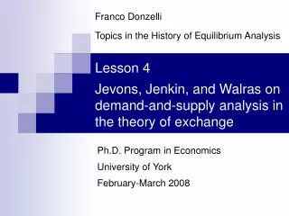
Franco Donzelli Topics in the History of Equilibrium Analysis. Lesson 4 Jevons, Jenkin, and Walras on demand-and-supply analysis in the theory of exchange. Ph.D. Program in Economics University of York February-March 2008. Introduction 1.

E N D
Franco Donzelli Topics in the History of Equilibrium Analysis Lesson 4Jevons, Jenkin, and Walras on demand-and-supply analysis in the theory of exchange Ph.D. Program in Economics University of York February-March 2008
Introduction 1 • W. Stanley Jevons develops his “theory of exchange” in: • “Brief Account” (1866) • Chapter 4 of The Theory of Political Economy (TPE), first edition (1871) • Chapter 4 of The Theory of Political Economy (TPE), second edition (1879) • In spite of Jevons’s insistence on the fundamental role of the so-called “laws of supply and demand”, no formal demand-and-supply analysis: • is actually employed by Jevons in the derivation of the theory; • can be actually deduced from the formal statement of the theory. • This is a mystery which has attracted some attention in the literature, but has not been adequately solved on theoretical grounds (White) Lesson 4 - Jevons, Jenkin, and Walras
Introduction 2 • A comparison with the theory of exchange put forward by two economists contemporary with Jevons, Léon Walras and Fleming Jenkin, can help unraveling this issue. • Léon Walras develops his theory of exchange in: • his first two mémoires: “Principe d’une théorie mathématique de l’échange” (1874) and “Equations de l’échange” (1877); • Section II of the first edition of the Eléments d’économie politique pure (Eléments)(1874). • Walras’s solution of the exchange problem rests on a fully-fledged demand-and supply analysis of the traders’ choices and behavior. • Since 1874, Walras repeatedly criticizes (in private correspondence and public contributions) Jevons’s approach to the theory of exchange, in particular the lack in it of a true and proper demand-and-supply analysis. Lesson 4 - Jevons, Jenkin, and Walras
Introduction 3 • Jevons does not react to Walras’s critical remarks: in particular he does not try to incorporate Walras’s implicit and explicit suggestions into the second edition of TPE. • Why? Perhaps because Walras’s remarks are made at a time when Jevons’s ideas have already taken a final shape, which cannot be easily modified. • But then why Jevons does not react to Jenkin’s remarks, that are advanced at a much earlier time (1868), when Jevons had not yet started writing TPE (1870)? • Fleeming Jenkin, an engineer-economist very active in the economic debates of the late 1860s and early 1870s, develops an almost complete microfounded demand-and-supply analysis and graphically solves the problem of equilibrium determination in an exchange economy in a series of two (or three) letters mailed to Jevons in 1868. Lesson 4 - Jevons, Jenkin, and Walras
Jevons’s theory of exchange: the conceptual apparatus 1 • In the first thirteen Sections of TPE Jevons discusses a two-trader, two-commodity, pure-exchange economy, that is an Edgeworth Box economyℰJ2x2 = {(ℝ2+, ui(‧), ωi)i=12} satisfying a few further specific assumptions concerning the traders’ endowments and utility functions: • the traders are “cornered”, with: ω1 = (ω̅1, 0), ω2 = (0, ω̅2) • each trader is characterized by a cardinal, additively separable utility function: satisfying the following restrictions on the signs of the first and second-order pure partial derivatives: Lesson 4 - Jevons, Jenkin, and Walras
Jevons’s theory of exchange: the conceptual apparatus 2 • Even if Jevons does not explicitly define the concept of Marginal Rate of Substitution, he implicitly uses it: • Even if Jevons’s model unambiguously refers to an Edgeworth Box economy, his verbal interpretation of the model is not free of major ambiguities. Lesson 4 - Jevons, Jenkin, and Walras
Jevons’s theory of exchange: the conceptual apparatus 3 • The first ambiguity has to do with Jevons's peculiar concept of "trading bodies", that are alternatively viewed as either individual traders, or representative agents, or "fictitious means". • The second ambiguity arises from Jevons's interpretation and use of the concepts of statics, dynamics and equilibrium: • after sharply distinguishing between statics and dynamics, and contending that the exchange problem ought be tackled from a purely statical point of view, Jevons is apparently willing to concede that the study of the equilibration process is not inconsistent with statics; • yet, after recognizing that a truly dynamic analysis would require integrating suitable differential equations describing the trading process over time, he ends up with endorsing a strictly “instantaneous” interpretation of the equilibrium concept. Lesson 4 - Jevons, Jenkin, and Walras
Jevons’s theory of exchange: the conceptual apparatus 4 • The third ambiguity is that surrounding the so-called “law of indifference”, which is initially viewed as the outcome of a market equilibration process taking place under stringent assumptions about the traders’ knowledge and information, but then reduced to an almost trivial truism in the only relevant application. • “Thus, from the self-evident principle, stated on p. 137, that there cannot, in the same market, at the same moment, be two different prices for the same uniform commodity, it follows that the last increments in an act of exchange must be exchanged in the same ratio as the whole quantities exchanged. [...] This result we may express by stating that the increments concerned in the process of exchange must obey the equation: Lesson 4 - Jevons, Jenkin, and Walras
Jevons’s theory of exchange: the conceptual apparatus 5 • The “law of indifference” is supposed to apply to an “act of exchange”, where “two commodities are bartered in the ratio of x₁ for x₂”. • Then the result is simply obtained by observing that "every mth part of x₁ is given for the mth part of x₂, [...] so that, at the limit, even an infinitely small part of x₁ must be exchanged for an infinitely small part of x₂, in the same ratio of the whole quantities", which is indeed a platitude. • An “act of exchange” involves two traders only. • The “law” holds “at one moment” and an “act of exchange” is “instantaneous” as well: Jevons should not speak of “the increments concerned in the process of exchange”. Lesson 4 - Jevons, Jenkin, and Walras
Jevons’s theory of exchange: a formal statement 1 • Jevons starts by assuming, “for a moment”, that the “[finite] ratio of exchange” between two commodities be “established” at a given level. • Under that provisional assumption, Jevons verbally arrives at the conclusion that the benefits from exchange for either trader cease when the ratio of each trader’s “degrees of utility” is equal to the inverse of the ‘differential’ “ratio of exchange” of the two commodities, which in turn is assumed to be equal to “the established [finite] ratio of exchange”. • The “point” so determined is called the “point of equilibrium” by Jevons. • First surprising omission: since the provisionally “established ratio of exchange” is generally not what would currently be called a competitive equilibrium “ratio”, the quantities of commodities that the traders want to exchange at Jevons’s “point of equilibrium” cannot generally be exchanged. Lesson 4 - Jevons, Jenkin, and Walras
Figure 1 Fig 1 Lesson 4 - Jevons, Jenkin, and Walras
Jevons’s theory of exchange: a formal statement 2 • But not a single word is uttered by Jevons about this eventuality and its possible consequences. • Similarly surprising is the diagram (Figure 5 of TPE) used to illustrate the verbal argument: one trader only; two superposed marginal utility curves, drawn under the assumption that “the ratio of exchange [...] be that of unit for unit, or 1 to 1”. • But, once again, nothing is said about the reason for selecting precisely that “ratio of exchange” or about the consequences of that selection, in the likely case the “1 to 1 ratio” were not what would currently be referred to as the competitive equilibrium “ratio”. • Then, taking for granted that equation (1) holds, Jevons eventually proceeds to determine the equilibrium conditions for his Edgeworth Box economy Lesson 4 - Jevons, Jenkin, and Walras
Exchange equilibrium in Jevons d*12 x*12 O2 tg α*= x*2/x*1= d*21/s*11 = s*22/d*12 = x*21/(ω̅1-x*11)= (ω̅2-x*22)/x*12 x*21 x*22 α* d*21 s*22 α* ω O1 x*11 Lesson 4 - Jevons, Jenkin, and Walras s*11
Jevons’s theory of exchange: a formal statement 3 • Jevons makes it clear that the subsequent discussion will concern what is supposed to hold in a “state of equilibrium”. • But the equilibrium concept is here used in a much stricter sense than before: he is actually referring to what would be termed nowadays a ‘competitive equilibrium’. • Letting x1* and x2∗ be the quantities of the two commodities traded in such a ‘competitive equilibrium’ state, x2∗/x1∗ turns out to be the competitive equilibrium ‘finite’ “ratio of exchange”. • Given the assumptions on the traders’ characteristics, one obviously has: x1*= s11*=d12* and x2* = d21* = s22*, where s11* = ω̅1 – x11* and d12* = x12∗ are the ‘competitive equilibrium’ quantities of commodity 1 respectively supplied by 1 and demanded by 2, while d21∗ = x21∗ and s22∗ = ω̅2 – x22∗ are the ‘competitive equilibrium’ quantities of commodity 2 respectively demanded by 1 and supplied by 2. Lesson 4 - Jevons, Jenkin, and Walras
Jevons’s theory of exchange: a formal statement 4 • Then, for any pair of differentials dx1∗ and dx2∗ such that dx2∗/dx1∗ = x2∗/x1∗, for trader 1 one has: or A similar condition holds for trader 2: Lesson 4 - Jevons, Jenkin, and Walras
Jevons’s theory of exchange: a formal statement 5 • Hence, by substituting (1) into both (2) and (3), one gets: which are Jevons’s “equations of exchange”, representing his fundamental result in the “theory of exchange”. • The way in which such “equations” are first obtained and then interpreted by Jevons prompts the following remarks. • In the first place, in deriving the “equations of exchange”, Jevons makes explicit use of the “law of indifference”, which holds only at a specified time instant. • Hence Jevons’s equilibrium concept must be given an “instantaneous” interpretation as well. Lesson 4 - Jevons, Jenkin, and Walras
Jevons’s theory of exchange: a formal statement 6 • In the second place, it should be stressed that Jevons’s argument is entirely couched in terms of the ‘competitive equilibrium’ values of the traded quantities of the two commodities, x₁∗ and x₂∗, from which Jevons directly derives the ‘finite’, ‘competitive equilibrium’ “ratio of exchange”, x₂∗/x₁∗, and indirectly also the ‘differential’ one, dx₂∗/dx₁∗, since the two “ratios” are assumed equal by virtue of the “law of indifference”. • Quantities or “ratios” different from the ‘competitive equilibrium’ ones are nowhere mentioned or even alluded to by Jevons in the development of his formal argument. • This explains why Jevons nowhere introduces, let alone discusses, an equation like: defining Edgeworth’s “contract curve”. Lesson 4 - Jevons, Jenkin, and Walras
Jevons’s theory of exchange: a formal statement 7 • In the third place, it remains to discuss what relationship, if any, can be established between Jevons's “theory of exchange”, as expressed by his “equations of exchange” (equations (4) above), and the so-called “laws of supply and demand”. • According to Jevons (1970, p. 143), his “theory is perfectly consistent with the laws of supply and demand”. • Yet such consistency boils down to a platitude: “We may regard x1 as the quantity demanded on one side and supplied on the other; similarly, x2 is the quantity supplied on the one side and demanded on the other. Now, when we hold the two equations to be simultaneously true, we assume that the x1 and x2 of one equation equal those of the other. The laws of supply and demand are thus a result of what seems to me the true theory of value or exchange.” (Jevons, 1970, pp. 143-4) Lesson 4 - Jevons, Jenkin, and Walras
Exchange equilibrium in Jevons d*12 x*12 O2 tg α*= x*2/x*1= d*21/s*11 = s*22/d*12 = x*21/(ω̅1-x*11)= (ω̅2-x*22)/x*12 x*21 x*22 α* d*21 s*22 α* ω O1 x*11 Lesson 4 - Jevons, Jenkin, and Walras s*11
Jevons’s theory of exchange: a formal statement 8 • Once the formal statement of the two-trader, two-commodity model is completed, Jevons tries to generalize his “equations of exchange” to economies with more than two traders and/or more than two commodities. • All his attempts rest on the assumption that: “the exchanges in the most complicated case may [...] always be decomposed into simple exchanges, and every exchange will give rise to two equations sufficient to determine the quantities involved.” (Jevons, 1970, p. 154) • Unfortunately, however, this assumption is unfounded. Hence, Jevons’s reductionist strategy ends up in a failure. • In spite of what he seems to suggest (1970, p. 154), Jevons is really unable to deal with traders who are not “cornered”. Lesson 4 - Jevons, Jenkin, and Walras
Jevons’s theory of exchange: a formal statement 9 • When he tries to put forward a theory of multilateral commodity exchanges, involving L > 2 commodities, he ends up with a set of L(L-1)/2 bilateral exchanges, each involving a pair of commodities and each viewed as independent of the others, so that the L(L-1)/2 “ratios of exchange”, obtained by applying the simple “equations of exchange” of Jevons’s simple two-commodity model, do not satisfy the Cournot-Walras arbitrage conditions. • Three main gaps in Jevons’s “theory of exchange”: • the price concept is almost entirely neglected and no serious demand-and-supply analysis is developed; • the equation of Edgeworth's “contract curve” is missing • no possible extension beyond the narrow boundaries of the two-trader, two-commodity model. Lesson 4 - Jevons, Jenkin, and Walras
Walras’s pure-exchange, two-commodity model 1 • Walras discusses a pure-exchange, two-commodity economy ℰW2xI = {(ℝ2+, ui(‧), ωi)i=1I}, with I ≥ 2, satisfying a few further specific assumptions concerning the traders’ endowments and utility functions: • the traders are “cornered”, with: ωi = (ω1i, 0), with ω1i > 0, for i = 1, …, I’, with I’ ≥ 1, and ωi = (0, ω2i), with ω2i > 0, for i = I’+1, …, I, with I > I’; • each trader is characterized by a cardinal, additively separable utility function, satisfying restrictions on the signs of the first and second-order pure partial derivatives similar to those assumed by Jevons. • Let p = (p12 ,1) ∈ ℝ2++ be the price system, expressed in terms of commodity 2 taken as the numeraire. • For all p = (p12 ,1) ∈ ℝ2++, the optimization problem to be solved by trader i can be written as: Lesson 4 - Jevons, Jenkin, and Walras
Walras’s pure-exchange, two-commodity model 2 • By solving this system, one obtains the individual demand and supply functions for the two commodities for each trader: for i = 1, …, I’, and for i = I’ + 1, …I. Lesson 4 - Jevons, Jenkin, and Walras
Walras’s pure-exchange, two-commodity model 3 • Then, by aggregating over the traders, one obtains the aggregate demand and supply functions for both commodities, from which one can get the excess demand functions: • By equating to zero the excess demand functions, one obtains the market clearing equations, one for each commodity: • Finally, by solving either equation, one obtains the Walrasian competitive equilibrium relative price, p12W. Lesson 4 - Jevons, Jenkin, and Walras
Walras’s pure-exchange, two-commodity model 4 • The solution thus arrived at is for Walras the “mathematical” (either “analytical” or “geometrical”) solution. • But, according to Walras, such solution is also concretely determined “on the market”, by means of the well-known tâtonnement process. • In the present case, the process will consist in the adjustment of the only one independent relative price, p12: p12 increases or decreases, according to whether z1(p12) is greater or less than zero, and the process goes on until the equilibrium price, p12W, is eventually reached. • With his model of a pure-exchange two-commodity economy, Walras arrives at results partially similar to those arrived at by Jevons a few years before with his “theory of exchange”. • This partial similarity, on the other hand, is explicitly recognized by both of them - with many a qualification on Walras's side - in the well-known exchange of correspondence taking place in May 1874. Lesson 4 - Jevons, Jenkin, and Walras
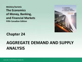
Exchange equilibrium in Walras d’12 x’12 x*12 O2 tg α’ = p’12= = d’21/s’11 = = s’22 /d’12 < tg α* = p*12 α* x*21 x*22 x’22 s’22 α* x’21 α’ d’21 ω O1 x*11 x’11 Lesson 4 - Jevons, Jenkin, and Walras s’11
Walras’s critique of Jevons’s theory of exchange 1 • Yet, in spite of the similarities in some of the results eventually obtained, not only does Walras’s overall approach significantly differ from Jevons’s, but the former’s exchange models also prove to be a potentially much richer theory than the latter's “theory of exchange”. • The fundamental difference between the two approaches lies in the different interpretation of the perfectly competitive hypothesis: the ‘Perfect Competition Assumption’ means for Walras, but not for Jevons, that the traders make their optimizing choices by taking prices as given parameters. • As Walras himself clearly points out (1988, p. 253, 2-5), in his exchange models Walras takes the “prix”, instead of Jevons’s “quantitités éxchangées”, “comme inconnues du problème”. • Thereby, he is able to extensively generalize the version of Jevons's “law of indifference” which is effectively employed by the latter in his “theory of exchange”, and which, as has been shown above, is really nothing more than a truism. Lesson 4 - Jevons, Jenkin, and Walras
Walras’s critique of Jevons’s theory of exchange 2 • What Walras actually resorts to in building his exchange models is a much more general “law”, that might be called the “Law of One Price”: at any given instant, one and the same price system is simultaneously announced to all traders, both at equilibrium and out of equilibrium. • Yet, out of equilibrium not all the chosen trading plans can be actually carried out. But this implies that some mentalistic concepts for which no observable counterpart can be found, such as the trading plans chosen by at least some traders when the economy is out of equilibrium, necessarily enter Walras’s exchange models. • Nothing similar can instead be found in Jevons’s “theory of exchange”: for, in this case, prices are never announced to traders, nor disequilibrium trading plans are ever explicitly taken into account. Lesson 4 - Jevons, Jenkin, and Walras
Walras’s critique of Jevons’s theory of exchange 3 • No prices and no trades other than the ‘competitive equilibrium’ ones, which are all observable magnitudes, appear in Jevons’s “equations”, which, as we have seen, are derived under the assumption that the economy already is “in an equilibrium state”. • Walras can immediately aggregate the traders’ optimal trading plans, irrespective of their number, and can consequently define the aggregate demand and supply functions for each commodity without any difficulty. • As Walras rightly points out (1993, p. 50), such functions cannot instead be obtained in Jevons’s case, due to the latter’s inability to take prices as the “inconnues du problème” and his related refusal to deal with unobservables. Lesson 4 - Jevons, Jenkin, and Walras
Walras’s critique of Jevons’s theory of exchange 4 • Walras, unlike Jevons, can extend his two-commodity model with “cornered” traders to a multi-commodity model with traders characterized by arbitrary endowments. • Finally, with his theory of the tâtonnement, Walras is apparently able to provide an answer to the issue of equilibrium attainment, an issue that had been left by Jevons in a state of ambiguity and confusion. • Yet Walras’s approach is far from unobjectionable: after Bertrand’s critique (1883), Walras is led to explicitly introduce a ‘No-Trade-Out-Of-Equilibrium Assumption’, which turns the tâtonnement process in the exchange models into a purely virtual process in ‘logical’ time, over which nothing observable is allowed to take place. Lesson 4 - Jevons, Jenkin, and Walras
Walras’s critique of Jevons’s theory of exchange 5 • Walras’s criticism of Jevons’s alleged shortcomings is quite explicit: “Je ne vois pas non plus que vous [...] fondiez [l'équation d'échange] sur la considération de satisfaction maximum, qui est pourtant si simple et si claire. Je ne vois pas non plus que vous en tiriez l'équation de la demand effective en fonction du prix, qui s'en déduit si aisément, et qui est si essentielle à la solution du problème de la détermination des prix d'équilibre.” (Walras, 1993, p. 50) • Yet, Jevons does not react to Walras’s critique. • One possible explanation is that it comes too late. • Yet, this is not a satisfactory explanation of Jevons’s silence: for Jevons had not apparently reacted to the critical remarks made by Jenkin in 1868 against the summary of Jevons’s theory put forward in the “Brief Account”. Lesson 4 - Jevons, Jenkin, and Walras
Jenkin on demand-and-supply analysis 1 • Jenkin's contribution essentially consists in an almost complete theory of both the derivation of the traders’ individual demand and supply curves from their marginal utility curves, and the graphical determination of a competitive equilibrium along quasi-Walrasian lines. • Not a single piece of the notable demand-and-supply apparatus put forward by Jenkin in his correspondence with Jevons finds its way into the latter’s later writings, including the two editions of TPE published during Jevons's lifetime. • Jenkin might have played with respect to Jevons a role similar to that played by Paul Piccard with respect to Walras. • But, while Walras is eager to exploit the new conceptual and analytical tools made available by Piccard in order to erect upon them his whole theoretical system, Jevons, instead, is not prepared to accept Jenkin's gift, also because that gift, unlike Piccard's, is partly poisonous. Lesson 4 - Jevons, Jenkin, and Walras
Figures 1, 2 Fig. 1 Fig. 2 Lesson 4 - Jevons, Jenkin, and Walras
Figures 3, 4 Fig. 3 Fig. 4 Lesson 4 - Jevons, Jenkin, and Walras
Figures 5, 6, 7 Fig. 5 Fig. 6 Fig. 7 Lesson 4 - Jevons, Jenkin, and Walras
Jenkin on demand-and-supply analysis 2 • The fact is that neither Jenkin, nor, to an even greater degree, Jevons himself are willing to bear the logical consequences of adopting an approach to the solution of the equilibrium determination problem in a pure-exchange economy that will later come to be known as the Walrasian demand-and-supply, or excess-demand, approach. • When in a pure-exchange, two-commodity model the traders are assumed to behave as competitive utility maximizers, three consequences necessarily follow: 1) at a given 'relative price' (or "ratio of exchange", or "rate of exchange"), the traders choose unobservable trade plans, typically unexecutable, which can be turned into observable, executable trades only at equilibrium; Lesson 4 - Jevons, Jenkin, and Walras
Jenkin on demand-and-supply analysis 3 2) the adjustment process towards equilibrium is brought about by progressively changing the ‘relative price’ in conformity to the usual price adjustment rule, according to which the change in the ‘relative price’ is a sign-preserving function of the aggregate excess-demand for the corresponding commodity; 3) the price change cannot itself be the product of the individual traders’ choices, but can only be effected by an objective mechanism, pursuing a superindividual aim. • Walras, after some uncertainties and oscillations, eventually accepts the rules of the competitive game. • As to the first rule, Jenkin’s stance is peculiar: for he accepts the competitive idea that the traders make their choices by taking the ‘relative price’ as a fixed parameter, but he does not accept the consequent requirement that no trades be carried out at disequilibrium ‘prices’. Lesson 4 - Jevons, Jenkin, and Walras
Jenkin on demand-and-supply analysis 4 On the contrary, according to Jenkin, plans must always be carried out, even out of equilibrium. But then he is forced to concoct an explanation for disequilibrium behavior, which explains his adoption of the “short-side rule”. • As to the adjustment process, Jenkin never accepts the idea that there exists an objective mechanism, moreover of a virtual type, which is at work in the economy. For him, the driving force of the adjustment process must lie in the subjective motivations of the individual members of the economy. But no such set of concurrent subjective motivations can possibly exist in an Edgeworth Box economy which is such as to lead the traders to jointly change the ‘relative price’ in a definite direction. Lesson 4 - Jevons, Jenkin, and Walras
Jevons on demand-and-supply analysis 1 • Given Jenkin’s negative conclusions about the possibility of buttressing Jevons’s “exchange equations” with a demand-and-supply analysis of the Walrasian type, it is not surprising that Jevons should not feel encouraged to exploit to his advantage the tools provided by his correspondent. • But the reasons underlying Jevons’s refusal to adopt a Walrasian or quasi-Walrasian approach to equilibrium determination in the theory of exchange are probably even more basic than those leading Jenkin to doubt of the usefulness of that approach. • For Jevons, in fact, the very distinction between a trade plan and an “act of trade” is unconceivable. • All trades of which one can legitimately speak are the observable outcome of bilateral bargains involving two traders at a time: there is no such thing as a trade plan, disconnected from an “act of trade”, which can in principle be carried out. Lesson 4 - Jevons, Jenkin, and Walras
Jevons on demand-and-supply analysis 2 • In short, no unobservable counterfactuals are allowed for in Jevons’s theory of exchange. • This has to do with the physicalist standpoint endorsed by Jevons: as in mechanics the motion of a material point in ordinary space can be obtained by integrating its velocity function w.r.t. time, so in an Edgeworth box economy the ‘trajectory’ described in the space of allocations by the commodity holdings of two traders can (or at least should) be obtained by integrating the ‘differential’ “ratio of exchange” between the two commodities. • The mechanical analogy is grossly misleading, yet it reveals the source of Jevons’s hostility towards unobservable counterfactuals. • But the distinction between trade plans and “acts of trade” as well as the use of unobservables and counterfactuals are crucial for the Walrasian type of demand-and-supply analysis, which is therefore precluded to Jevons. Lesson 4 - Jevons, Jenkin, and Walras
Figures 1 Fig 1 Fig. 2 Lesson 4 - Jevons, Jenkin, and Walras
Figures 2 Fig 3 Fig. 4 Lesson 4 - Jevons, Jenkin, and Walras
Figures 3 Fig 5 Fig. 6 Fig. 7 Lesson 4 - Jevons, Jenkin, and Walras
Exchange equilibrium in Jevons d*12 x*12 O2 tg α*= x*2/x*1= d*21/s*11 = s*22/d*12 = x*21/(ω̅1-x*11)= (ω̅2-x*22)/x*12 x*21 x*22 α* d*21 s*22 α* ω O1 x*11 Lesson 4 - Jevons, Jenkin, and Walras s*11
Exchange equilibrium in Walras d’12 x’12 x*12 O2 tg α’ = p’12= = d’21/s’11 = = s’22 /d’12 < tg α* = p*12 α* x*21 x*22 x’22 s’22 α* x’21 α’ d’21 ω O1 x*11 x’11 Lesson 4 - Jevons, Jenkin, and Walras s’11