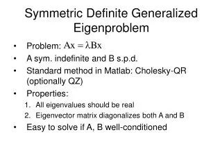
Symmetric Definite Generalized Eigenproblem
Symmetric Definite Generalized Eigenproblem. Problem: A sym. indefinite and B s.p.d. Standard method in Matlab: Cholesky-QR (optionally QZ) Properties: All eigenvalues should be real Eigenvector matrix diagonalizes both A and B Easy to solve if A, B well-conditioned.

Symmetric Definite Generalized Eigenproblem
E N D
Presentation Transcript
Symmetric Definite Generalized Eigenproblem • Problem: • A sym. indefinite and B s.p.d. • Standard method in Matlab: Cholesky-QR (optionally QZ) • Properties: • All eigenvalues should be real • Eigenvector matrix diagonalizes both A and B • Easy to solve if A, B well-conditioned
Motivation: Animation • Goal: create interactive animations of deforming objects • Use finite element method • Problem: solving the PDEs is slow. • Solution: Linear Algebra! • Kris Hauser, Chen Shen, James O’Brien • Interactive Deformation using Modal Analysis with Constraints • Graphics Interface 2003 • Diagonalize the system to create a set of uncoupled differential equations (modes). • Extract the most important modes from the system, and simulate only those. • The eigenvectors with the largest eigenvalues describe the most important modes. • Perhaps only a dozen, out of thousands, really matter.
The Eigenproblem The FEM model gives us a system of ODEs Which can be simplified to use two matrices These matrices are symmetric positive definite Modal analysis is a generalized eigenproblem
Conditioning • We want to apply this method to any mesh we happen to throw at it. • Some models lead to ill-conditioned matrices. • Depends on shape of elements • Figure by Jonathan Shewchuk, from “What is a good finite element”
Davies, Higham and Tisseur • Cholesky on B • Jacobi’s method to solve eigenproblem • Iterative refinement based on Newton’s • Claim: new error bound, potentially better
Error bounds and numerical results • Old bound: • Want to get rid of • New bound: • Where
Newton’s method is applied to the equivalent problem • They first present an algorithm for iterative refinement, cost O(n^3) • Improved algorithm is O(n^2), but at the cost of “less frequent and less rapid convergence”
Numerical Results • n=20, A=I, B=RTR (R is a Kahan matrix) • Plot of eigenvalues vs. backward error of the eigenpairs:
Chandrasekaran • Claim: new algorithm is numerically stable and “efficient” which satisfies both properties • All eigenvalues should be real • Eigenvector matrix diagonalizes both A and B • Idea: Find C such that • Where and are diagonal • Eigenvalues: • Eigenvectors:
Error Bounds and numerical results • Error bound for an eigenvalue/vector pair: • Numerical experiment: • A and B are 5x5 • Matlab’s QZ algorithm gives large imaginary parts • The algorithm in this paper returns all eigenvalues and eigenvectors to full backward accuracy