CIRCULAR LINKED LIST
CIRCULAR LINKED LIST.


CIRCULAR LINKED LIST
E N D
Presentation Transcript
Circular Linked List- A circular linked list is a linked list in which last element or node of the list points to first node. For non-empty circular linked list, there are no NULL pointers. The memory declarations for representing the circular linked lists are the same as for linear linked lists. All operations performed on linear linked lists can be easily extended to circular linked lists with following exceptions: • While inserting new node at the end of the list, its next pointer field is made to point to the first node. • While testing for end of list, we compare the next pointer field with address of the first node Circular linked list is usually implemented using header linked list. Header linked list is a linked list which always contains a special node called the header node, at the beginning of the list. This header node usually contains vital information about the linked list such as number of nodes in lists, whether list is sorted or not etc. Circular header lists are frequently used instead of ordinary linked lists as many operations are much easier to state and implement using header lists
This comes from the following two properties of circular header linked lists: • The null pointer is not used, and hence all pointers contain valid addresses • Every (ordinary ) node has a predecessor, so the first node may not require a special case.
Algorithm: (Traversing a circular header linked list) This algorithm traverses a circular header linked list with START pointer storing the address of the header node. • Step 1: Set PTR:=LINK[START] • Step 2: Repeat while PTR≠START: Apply PROCESS to INFO[PTR] Set PTR:=LINK[PTR] [End of Loop] • Step 3: Return
Searching a circular header linked list • Algorithm: SRCHHL(INFO,LINK,START,ITEM,LOC) • This algorithm searches a circular header linked list • Step 1: Set PTR:=LINK[START] • Step 2: Repeat while INFO[PTR]≠ITEM and PTR≠START: Set PTR:=LINK[PTR] [End of Loop] • Step 3: If INFO[PTR]=ITEM, then: Set LOC:=PTR Else: Set LOC:=NULL [End of If structure] • Step 4: Return
Deletion from a circular header linked list Algorithm: DELLOCHL(INFO,LINK,START,AVAIL,ITEM) This algorithm deletes an item from a circular header linked list. • Step 1: CALL FINDBHL(INFO,LINK,START,ITEM,LOC,LOCP) • Step 2: If LOC=NULL, then: Write: ‘item not in the list’ Exit • Step 3: Set LINK[LOCP]:=LINK[LOC] [Node deleted] • Step 4: Set LINK[LOC]:=AVAIL and AVAIL:=LOC • [Memory retuned to Avail list] • Step 5: Return
Algorithm: FINDBHL(NFO,LINK,START,ITEM,LOC,LOCP) This algorithm finds the location of the node to be deleted and the location of the node preceding the node to be deleted • Step 1: Set SAVE:=START and PTR:=LINK[START] • Step 2: Repeat while INFO[PTR]≠ITEM and PTR≠START Set SAVE:=PTR and PTR:=LINK[PTR] [End of Loop] • Step 3: If INFO[PTR]=ITEM, then: Set LOC:=PTR and LOCP:=SAVE Else: Set LOC:=NULL and LOCP:=SAVE [End of If Structure] • Step 4: Return
Insertion in a circular header linked list Algorithm: INSRT(INFO,LINK,START,AVAIL,ITEM,LOC) This algorithm inserts item in a circular header linked list after the location LOC • Step 1:If AVAIL=NULL, then Write: ‘OVERFLOW’ Exit • Step 2: Set NEW:=AVAIL and AVAIL:=LINK[AVAIL] • Step 3: Set INFO[NEW]:=ITEM • Step 4: Set LINK[NEW]:=LINK[LOC] Set LINK[LOC]:=NEW • Step 5: Return
Insertion in a sorted circular header linked list Algorithm: INSSRT(INFO,LINK,START,AVAIL,ITEM) This algorithm inserts an element in a sorted circular header linked list Step 1: CALL FINDA(INFO,LINK,START,ITEM,LOC) Step 2: If AVAIL=NULL, then Write: ‘OVERFLOW’ Return Step 3: Set NEW:=AVAIL and AVAIL:=LINK[AVAIL] Step 4: Set INFO[NEW]:=ITEM Step 5: Set LINK[NEW]:=LINK[LOC] Set LINK[LOC]:=NEW Step 6: Return
Algorithm: FINDA(INFO,LINK,ITEM,LOC,START) This algorithm finds the location LOC after which to insert • Step 1: Set PTR:=START • Step 2: Set SAVE:=PTR and PTR:=LINK[PTR] • Step 3: Repeat while PTR≠START If INFO[PTR]>ITEM, then Set LOC:=SAVE Return Set SAVE:=PTR and PTR:=LINK[PTR] [End of Loop] • Step 4: Set LOC:=SAVE • Step 5: Return
One of the most important application of Linked List is representation of a polynomial in memory. Although, polynomial can be represented using a linear linked list but common and preferred way of representing polynomial is using circular linked list with a header node. • Polynomial Representation: Header linked list are frequently used for maintaining polynomials in memory. The header node plays an important part in this representation since it is needed to represent the zero polynomial. • Specifically, the information part of node is divided into two fields representing respectively, the coefficient and the exponent of corresponding polynomial term and nodes are linked according to decreasing degree. List pointer variable POLY points to header node whose exponent field is assigned a negative number, in this case -1. The array representation of List will require three linear arrays as COEFF, EXP and LINK. For example: • P(x)= 2x8-5x7-3x2+4 can be represented as:
POLY HEADER NODE WITH EXP -1 AND COEFF 0 0 -1 2 8 -5 7 -3 2 4 0 CIRCULAR HEADER LINEKD LIST REPRESENTATION OF2x8-5x7-3x2+4
Addition of polynomials using linear linked list representation for a polynomial
Algorithm:ADDPOLY( COEFF, POWER, LINK, POLY1, POLY2, SUMPOLY, AVAIL) This algorithm adds the two polynomials implemented using linear linked list and stores the sum in another linear linked list. POLY1 and POLY2 are the two variables that point to the starting nodes of the two polynomials. Step 1: Set SUMPOLY:=AVAIL and AVAIL:=LINK[AVAIL] Step 2: Repeat while POLY1 ≠ NULL and POLY2≠NULL: If POWER[POLY1]>POWER[POLY2],then: Set COEFF[SUMPOLY]:=COEFF[POLY1] Set POWER[SUMPOLY]:=POWER[POLY1] Set POLY1:=LINK[POLY1] Set LINK[SUMPOLY]:=AVAIL and AVAIL:=LINK[AVAIL] Set SUMPOLY:=LINK[SUMPOLY] Else If POWER[POLY2]>POWER[POLY1], then: Set COEFF[SUMPOLY]:=COEFF[POLY2] Set POWER[SUMPOLY]:=POWER[POLY2] Set POLY2:=LINK[POLY2] Set LINK[SUMPOLY]:=AVAIL and AVAIL:=LINK[AVAIL] Set SUMPOLY:=LINK[SUMPOLY]
Else: Set COEFF[SUMPOLY]:=COEFF[POLY1]+COEFF[POLY2] Set POWER[SUMPOLY]:=POWER[POLY1] Set POLY1:=LINK[POLY1] Set POLY2=LINK[POLY2] Set LINK[SUMPOLY]:=AVAIL and AVAIL:=LINK[AVAIL] Set SUMPOLY:=LINK[SUMPOLY] [End of If structure] [End of Loop] • Step3: If POLY1=NULL , then: Repeat while POLY2≠NULL Set COEFF[SUMPOLY]:=COEFF[POLY2] Set POWER[SUMPOLY]:=POWER[POLY2] Set POLY2:=LINK[POLY2] Set LINK[SUMPOLY]:=AVAIL and AVAIL:=LINK[AVAIL] Set SUMPOLY:=LINK[SUMPOLY] [End of Loop] [End of If Structure]
Step 4: If POLY2=NULL, then: Repeat while POLY1≠NULL Set COEFF[SUMPOLY]:=COEFF[POLY1] Set POWER[SUMPOLY]:=POWER[POLY1] Set POLY1:=LINK[POLY1] Set LINK[SUMPOLY]:=AVAIL and AVAIL:=LINK[AVAIL] Set SUMPOLY:=LINK[SUMPOLY] [End of Loop] [End of If Structure] Step 5: Set LINK[SUMPOLY]:=NULL Set SUMPOLY:=LINK[SUMPOLY] Step 6: Return
Addition of polynomials using circular header linked list representation for polynomials
Algorithm: ADDPOLY( COEFF, POWER, LINK, POLY1,POLY2, SUMPOLY, AVAIL) This algorithm finds the sum of two polynomials implemented using header circular linked lists. POLY1 and POLY2 contain the addresses of header nodes of two polynomials and SUMPOLY is the circular header linked list storing the terms of sum of two polynomials Step 1: Set HEADER:=AVAIL and AVAIL:=LINK[AVAIL] Step 2: Set SUMPOLY:=HEADER Set LINK[SUMPOLY ]:=AVAIL and AVAIL:=LINK[AVAIL] Set SUMPOLY:=LINK[SUMPOLY] Step 3: Set START1:=POLY1 and START2:=POLY2 Set POLY1:=LINK[START1] and POLY2:=LINK[START2] Step 4: Repeat while POLY1 ≠ START1 and POLY2≠START2: If POWER[POLY1]>POWER[POLY2],then: Set COEFF[SUMPOLY]:=COEFF[POLY1] Set POWER[SUMPOLY]:=POWER[POLY1] Set POLY1:=LINK[POLY1] Set LINK[SUMPOLY]:=AVAIL and AVAIL:=LINK[AVAIL] Set SUMPOLY:=LINK[SUMPOLY] Else If POWER[POLY2]>POWER[POLY1], then: Set COEFF[SUMPOLY]:=COEFF[POLY2] Set POWER[SUMPOLY]:=POWER[POLY2] Set POLY2:=LINK[POLY2] Set LINK[SUMPOLY]:=AVAIL and AVAIL:=LINK[AVAIL] Set SUMPOLY:=LINK[SUMPOLY]
Else: Set COEFF[SUMPOLY]:=COEFF[POLY1]+COEFF[POLY2] Set POWER[SUMPOLY]:=POWER[POLY1] Set POLY1:=LINK[POLY1] Set POLY2=LINK[POLY2] Set LINK[SUMPOLY]:=AVAIL and AVAIL:=LINK[AVAIL] Set SUMPOLY:=LINK[SUMPOLY] [End of If structure] [End of Loop] • Step5: If POLY1=START1 , then: Repeat while POLY2≠ START2 Set COEFF[SUMPOLY]:=COEFF[POLY2] Set POWER[SUMPOLY]:=POWER[POLY2] Set POLY2:=LINK[POLY2] Set LINK[SUMPOLY]:=AVAIL and AVAIL:=LINK[AVAIL] Set SUMPOLY:=LINK[SUMPOLY] [End of Loop] [End of If Structure]
Step 6: If POLY2=START2, then: Repeat while POLY1≠START1 Set COEFF[SUMPOLY]:=COEFF[POLY1] Set POWER[SUMPOLY]:=POWER[POLY1] Set POLY1:=LINK[POLY1] Set LINK[SUMPOLY]:=AVAIL and AVAIL:=LINK[AVAIL] Set SUMPOLY:=LINK[SUMPOLY] [End of Loop] [End of If Structure] Step 7: Set LINK[SUMPOLY]:=HEADER and SUMPOLY:=LINK[SUMPOLY] Step 8: Return
Multiplication of Polynomials using linear linked list representation for polynomials
Algorithm: MULPOLY( COEFF, POWER, LINK, POLY1, POLY2, PRODPOLY, AVAIL) This algorithm multiplies two polynomials implemented using linear linked list. POLY1 and POLY2 contain the addresses of starting nodes of two polynomials. The result of multiplication is stored in another linked list whose starting node is PRODPOLY Step 1: Set PRODPOLY:=AVAIL and AVAIL:=LINK[AVAIL] Set START:=PRODPOLY Step 2: Repeat while POLY1 ≠ NULL Step 3:Repeat while POLY2≠NULL: Set COEFF[PRODPOLY]:=COEFF[POLY1]*COEFF[POLY2] Set POWER[PRODPOLY]:=POWER[POLY1]+POWER[POLY2] Set POLY2:=LINK[POLY2] Set LINK[PRODPOLY]:=AVAIL and AVAIL:=LINK[AVAIL] Set PRODPOLY:=LINK[PRODPOLY] [End of step 4 loop] Set POLY1:=LINK[POLY1] [End of step 3 loop] Step 4 Set LINK[PRODPOLY]:=NULL and PRODPOLY:=LINK[PRODPOLY] Step 5: Return
Algorithm: MULPOLY( COEFF, POWER, LINK, POLY1, POLY2, PRODPOLY, AVAIL) This algorithm finds the product of two polynomials implemented using header circular linked list. POLY1 and POLY2 contain addresses of header nodes of two polynomials. The result of multiplication is stored in another header circular linked list. Step 1: Set HEADER:=AVAIL and AVAIL:=LINK[AVAIL] Step 2: Set PRODPOLY :=HEADER Set LINK[PRODPOLY ]:=AVAIL and AVAIL:=LINK[AVAIL] Set PRODPOLY:=LINK[PRODPOLY] Step 3: Set START1:=POLY1 and START2:=POLY2 Set POLY1:=LINK[START1] and POLY2:=LINK[START2] Step 4: Repeat while POLY1 ≠ START1 Step 5: Repeat while POLY2≠ START2 Set COEFF[PRODPOLY]:=COEFF[POLY1]*COEFF[POLY2] Set POWER[PRODPOLY]:=POWER[POLY1]+POWER[POLY2] Set POLY2:=LINK[POLY2] Set LINK[PRODPOLY]:=AVAIL and AVAIL:=LINK[AVAIL] Set PRODPOLY:=LINK[PRODPOLY] [End of Step 5 Loop] Set POLY1:=LINK[POLY1] [End of Step 4 Loop] Step 6: Set LINK[PRODPOLY]:=HEADER and PRODPOLY:=LINK[PRODPOLY] Step 7: Return
Doubly Linked List: Two-way List • A two-way list is a linear linked list which can be traversed in two directions: in usual forward direction from beginning of the list to end and in backward direction from end of list to the beginning. Thus, given the location LOC of a node N in list, one has immediate access to both the next node and the preceding node in the list. • Each node of a two-way list is divided into three parts: • An information field INFO which contains data of N • A pointer field FORW which contains the location of next node in the list • A pointer field BACK which contains the location of preceding node. The list also requires two list pointer variables FIRST which points to first node in the list and LAST which points to the last node in the list. Thus null pointer will appear in FORW field of last node in list and also in BACK field of first node in list.
LAST • Two way lists are maintained in memory by means of linear arrays in same way as one way list except that two pointer arrays , FORW and BACK , are required instead of one list pointer variable. The list AVAIL will still be maintained as a one-way list. FIRST FORW[PTR] BACK[PTR]
Operations on a Two-way list • Traversal • Algorithm: Traversal This algorithm traverses a two-way list. FORW and BACK are the two address parts of each node containing the address of next node and previous node respectively. INFO is the information part of each node. START contains the address of the first node Step 1: Set PTR:=START Step 2: Repeat while PTR≠ NULL Apply PROCESS to INFO[PTR] Step 3: Set PTR:=FORW[PTR] [End of Step 2 Loop] Step 4: Exit
Algorithm: SEARCH(INFO,FORW,BACK,ITEM,START,LOC) This algorithm searches the location LOC of ITEM in a two- way list and sets LOC=NULL if ITEM is not found in the list • Step 1: Set PTR:=START • Step 2: Repeat while PTR≠NULL and INFO[PTR]≠ITEM Set PTR:=FORW[PTR] [End of Loop] • Step 3: If INFO[PTR]=ITEM, then: Set LOC:=PTR Else: Set LOC:=NULL • Step 4: Return
Algorithm: DELETE(INFO,FROW,BACK,START,AVAIL,LOC) This algorithm deletes a node from a two-way list • Step 1: If LOC=START , then: START:=FORW[START] BACK[START]:=NULL Return • Step 2: [Delete node] Set FORW[BACK[LOC]]:=FORW[LOC] Set BACK[FORW[LOC]]:=BACK[LOC] • Step 3: [Returning node to AVAIL] Set FORW[LOC]:=AVAIL and AVAIL:=LOC • Step 4: Return
Algorithm:INSRT (INFO,FORW,BACK,START,AVAIL,LOCA, LOCB, ITEM) This algorithm inserts an item in a doubly linked list. LOCA and LOCB location of adjacent nodes A and B • Step 1: [OVERFLOW] If AVAIL=NULL, then: Write: OVERFLOW Return • Step 2: Set NEW:=AVAIL and AVAIL:=LINK[AVAIL] Set INFO[NEW]:=ITEM • Step 3: Set FORW[LOCA]:=NEW and BACK[NEW]:=LOCA Set FORW[NEW]:=LOCB and BACK[LOCB]:=NEW • Step 4: Return
BACK[PTR] NEW FORW[PTR]
Algorithm to copy the contents of one linked list to another • Algorithm: Copy (INFO,LINK,START,AVAIL) This algorithm copies the contents of one linked list to another. • Step 1: If AVAIL=NULL,then Write: ‘Overflow’ Return • Step 2: Set PTR:=START • Step 3: Set NEW:=AVAIL , START1:=NEW and AVAIL:=LINK[AVAIL] • Step 4: Repeat while PTR≠ NULL INFO[NEW]:=INFO[PTR] LINK[NEW]:=AVAIL and AVAIL:=LINK[AVAIL] NEW:=LINK[NEW] [End of Loop] • Step 5: Set LINK[NEW]:=NULL • Step 6: Return
Algorithm: Copy (INFO,LINK,START,START1) This algorithm copies the contents of one linked list to another. START AND START1 are the start pointers of two lists • Step 1: Set PTR:=START and PTR1:=START1 • Step 2: Repeat while PTR≠ NULL and PTR1 ≠ NULL INFO[PTR1]:=INFO[PTR] PTR1:=LINK[PTR1] PTR:=LINK[PTR] [End of Loop] • Step 3: If PTR=NULL and PTR1=NULL Return • Step 4:[Case when the list to be copied is still left] If PTR1=NULL,then PTR1: =AVAIL and AVAIL:=LINK[AVAIL] Repeat while PTR ≠ NULL INFO[PTR1]:=INFO[PTR] LINK[PTR1]:=AVAIL and AVAIL:=LINK[AVAIL] PTR1:=LINK[PTR1] [End of Loop] • Step 5: [Case when list to be copied is finished, Truncate the extra nodes] If PTR1 ≠NULL, then Set PTR1:=NULL [End of If structure] • Step 6: Return
Algorithm to insert a node after the kth node in the circular linked list • Algorithm: INSRT (INFO,LINK,START,AVAIL,K,ITEM) This algorithm inserts in a circular linked list after the kth node • Step 1: If AVAIL:=NULL, then Write: ‘OVERFLOW’ Return • Step 2: Set NEW:=AVAIL and AVAIL:=LINK[AVAIL] • Set INFO[NEW]:=ITEM • Step 3: Set PTR:=START and N:=1 • Step 4: If N=K, then Set LINK[NEW]:=LINK[PTR] Set LINK[PTR]:=NEW Return • Step 5: Set PTR:=LINK[PTR] and • Step 6: Repeat while N≠ K Set PTR:=LINK[PTR] and N:=N+1 [End of if structure] • Step 7: Set LINK[NEW]:=LINK[PTR] Set LINK[PTR]:=NEW • Step 8: Return
Algorithm to delete the kth node from a doubly linked list • Algorithm: Del (INFO,FORW,BACK,FIRST,LAST,AVAIL,K) This algorithm deletes the kth node • Step 1: Set N:=1 and PTR:=FIRST • Step 2: Set SAVE:=PTR and PTR:=FORW[PTR] • Step 3: Repeat while N≠ K Set SAVE:=PTR and PTR:=FORW[PTR] Set N:=N+1 [End of If structure] • Step 4: If N=K, then FORW[SAVE]:=FORW[PTR] BACK[FORW[PTR]]:=BACK[PTR] FORW[PTR]:=AVAIL and AVAIL:=PTR [End of If structure] • Step 5: Return
In computer science, garbage collection (GC) is a form of automatic memory management. The garbage collector, or just collector, attempts to reclaim garbage, or memory used by objects that will never be accessed or mutated again by the application. Garbage collection is often portrayed as the opposite of manual memory management, which requires the programmer to specify which objects to deallocate and return to the memory system. • The basic principle of how a garbage collector works is: • Determine what data objects in a program will not be accessed in the future • Reclaim the resources used by those objects . Reachability of an object • Informally, a reachable object can be defined as an object for which there exists some variable in the program environment that leads to it, either directly or through references from other reachable objects. More precisely, objects can be reachable in only two ways: • A distinguished set of objects are assumed to be reachable—these are known as the roots. Typically, these include all the objects referenced from anywhere in the call stack (that is, all local variables and parameters in the functions currently being invoked), and any global variables. • Anything referenced from a reachable object is itself reachable; more formally, reachability is a transitive closure .
The memory is traced for garbage collection using Tracing collectors OR SIMPLY COLLECTORS . Tracing collectors are called that way because they trace through the working set of memory. These garbage collectors perform collection in cycles. A cycle is started when the collector decides (or is notified) that it needs to reclaim storage, which in particular happens when the system is low on memory. The original method involves a naive mark-and-sweep in which the entire memory set is touched several times • In this method, each object in memory has a flag (typically a single bit) reserved for garbage collection use only. This flag is always cleared (counter-intuitively), except during the collection cycle. The first stage of collection sweeps the entire 'root set', marking each accessible object as being 'in-use'. All objects transitively accessible from the root set are marked, as well. Finally, each object in memory is again examined; those with the in-use flag still cleared are not reachable by any program or data, and their memory is freed. (For objects which are marked in-use, the in-use flag is cleared again, preparing for the next cycle.).
Moving vs. non-moving garbage Collection • Once the unreachable set has been determined, the garbage collector may simply release the unreachable objects and leave everything else as it is, or it may copy some or all of the reachable objects into a new area of memory, updating all references to those objects as needed. These are called "non-moving" and "moving" garbage collectors, respectively. • At first, a moving GC strategy may seem inefficient and costly compared to the non-moving approach, since much more work would appear to be required on each cycle. In fact, however, the moving garbage collection strategy leads to several performance advantages, both during the garbage collection cycle itself and during actual program execution
Stack- A stack is a linear data structure in which items may be added or removed only at one end . Accordingly, stacks are also called last-in-first-out or LIFO lists. The end at which element is added or removed is called the top of the stack. Two basic operations associated with stacks are : • Push- Term used to denote insertion of an element onto a stack. • Pop- Term used to describe deletion of an element from a stack. The order in which elements are pushed onto a stack is reverse of the order in which elements are popped from a stack
Representation of stacks • Stacks may be represented in memory in various ways usually by means of one-way list or a linear array In array representation of stack, stack is maintained by an array named STACK , a variable TOP which contains the location/index of top element of stack and a variable MAXSTK giving the maximum number of elements that can be held by the stack. The condition TOP=0 or TOP=NULL indicates that stack is empty. The operation of addition of an item on stack and operation of removing an item from a stack may be implemented respectively by sub algorithms, called PUSH and POP. Before executing operation PUSH on to a stack, one must first test whether there is room in the stack for the new item. If not, then we have the condition known as overflow. Analogously, in executing the POP operation, one must first test where there is an element in stack to be deleted. If not, then we have condition known as underflow.
Algorithm: PUSH (STACK,TOP,MAXSTK,ITEM) This algorithm pushes an item onto the stack array. TOP stores the index of top element of the stack and MAXSTK stores the maximum size of the stack. • Step 1: [Stack already filled] If TOP=MAXSTK, then: Write: ‘OVERFLOW’ Return • Step 2: Set TOP:=TOP+1 • Step 3: Set STACK[TOP]:=ITEM • Step 4: Return
Algorithm: POP(STACK,TOP,ITEM) This procedure deletes the top element of STACK array and assign it to variable ITEM • Step 1: If TOP=0,then: Write: ‘UNDERFLOW’ Return • Step 2: Set ITEM:=STACK[TOP] • Step 3: Set TOP:=TOP-1 • Step 4: Return
A stack represented using a linked list is also known as linked stack. The array based representation of stack suffers from following limitations: • Size of stack must be known in advance • Representing stack as an array prohibits the growth of stack beyond finite number of elements. In a linked list implementation of stack, each memory cell will contain the data part of the current element of stack and pointer that stores the address of its bottom element and the memory cell containing the bottom most element will have a NULL pointer
Push operation on linked list representation of stack • Algorithm: PUSH(INFO, LINK, TOP, ITEM, AVAIL) This algorithm pushes an element to the top of the stack Step 1: If AVAIL=NULL, then Write: ‘OVERFLOW’ Return Step 2: Set NEW:=AVAIL and AVAIL:=LINK[AVAIL] Step 3: Set INFO[NEW]:=ITEM Step 4: If TOP=NULL, then Set LINK[NEW]:=NULL Set TOP:=NEW Return Else: Set LINK[NEW]:=TOP Set TOP:=NEW Step 5: Return
POP operation on linked list representation of stack • Algorithm: POP(INFO, LINK, TOP, AVAIL) • This algorithm deletes an element from the top of the stack • Step 1: If TOP=NULL , then: Write: ‘UNDERFLOLW’ Return • Step 2: Set PTR:=TOP Set TOP:=LINK[TOP] Write: INFO[PTR] • Step 3: Set LINK[PTR]:=AVAIL and AVAIL:=PTR • Step 4: Return
Application of stack • Evaluation of arithmetic expression. • For most common arithmetic operations, operator symbol is placed between its operands. This is called infix notation of an expression. To use stack to evaluate an arithmetic expression, we have to convert the expression into its prefix or postfix notation. • Polish notation , refers to the notation in which operator symbol is placed before its two operands. This is also called prefix notation of an arithmetic expression. The fundamental property of polish notation is that the order in which operations are to be performed is completely determined by positions of operators and operands in expression. Accordingly, one never needs parentheses when writing expression in polish notation. • Reverse Polish notation refers to notation in which operator is placed after its two operands. This notation is frequently called postfix notation. Examples of three notations are:
INFIX NOTATION: A+B • PREFIX OR POLISH NOTATION: +AB • POSTFIX OR REVERSE POLISH NOATATION: AB+ • Convert the following infix expressions to prefix and postfix forms • A+(B*C) • (A+B)/(C+D) • Prefix: +A*BC Postfix: A BC*+ • Prefix: / +AB+CD Postfix: AB+CD+/