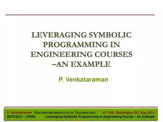
LEVERAGING SYMBOLIC PROGRAMMING IN ENGINEERING COURSES –AN EXAMPLE
LEVERAGING SYMBOLIC PROGRAMMING IN ENGINEERING COURSES –AN EXAMPLE. P. Venkataraman. Todays Presentation. Advantages of Symbolic Programming In Instruction Minimum Command Set Some Examples Field Description Substantial Derivatives Stream Function and Velocity Potential Integral Equation

LEVERAGING SYMBOLIC PROGRAMMING IN ENGINEERING COURSES –AN EXAMPLE
E N D
Presentation Transcript
LEVERAGING SYMBOLIC PROGRAMMING IN ENGINEERING COURSES –AN EXAMPLE P. Venkataraman
Todays Presentation • Advantages of Symbolic Programming In Instruction • Minimum Command Set • Some Examples • Field Description • Substantial Derivatives • Stream Function and Velocity Potential • Integral Equation • Conclusion
Advantages of Symbolic Programming In Instruction 1. Reinforces calculus ( a distinct weakness in a significant fraction of students) Examples are from the basic course Aerodynamics (Junior/Senior year) • Students have to • Differentiate • Integrate • Deal with vectors and matrices • Solve algebraic equations • Solve ordinary differential equations • Deal with nonlinear problems • Understand partial differential equations • Use numerical computation • Deal with integral equations • Solve matrix equations.
Advantages of Symbolic Programming In Instruction 2. Allows easy incorporation of graphical solution( leads to better understanding) The software used is MATLAB as it is a resource available both to faculty and the students in the College of Engineering Software is encouraged in other courses in the department Software allows easy mix of numeric and symbolic computation 3. Easier to deploy than traditional numeric programming ( makes it easy to incorporate in lectures and almost no leaning curve ) 4. Access to important geometric and trigonometric identities ( allows us to recover all the mathematical knowledge students should posses but have seriously forgotten )
The Minimal Command Set This small set of commands Sufficient for all courses that uses mathematics in small or significant amounts Does not require any training. Even a novice to MATLAB can use symbolic computation effectively Some challenges Patience (symbolic computations are a little slower ) Results are sometimes long mathematical expressions difficult to understand or decode A little experience in debugging (learning to deal with unexpected results )
The Minimal Command Set syms - define symbolic variables subs - substitute values for variables in expressions double – convert to a real number solve – solves algebraic equations dsolve – solves ordinary differential equations diff – differentiates an expression int – integrates an expression ezplot– 2D plot of a symbolic expression ezcontour – contour plot of a symbolic expression
Some Examples Field Description syms x y% definitions u = 10 + 5*(x+2)/((x+2)^2+y^2)- 5*(x-2)/((x-2)^2+y^2) v = 5*y/((x+2)^2+y^2)-5*y/((x-2)^2+y^2) A steady, 2D, incompressible, irrotational velocity field % graphics (contour u(x,y) ezcontourf(u,[-4 4 -4 4],20) grid, colorbar
Some Examples Field Description figure %graphics–velocity vectors [X, Y] = … meshgrid(-4:.4:4,-4:.4:4); U = subs(u, {x y}, {X,Y}); V = subs(v, {x y}, {X,Y}); quiver(X, Y, U, V) grid
Some Examples Substantial Derivative syms x y% definitions u = 10 + 5*(x+2)/((x+2)^2+y^2)- 5*(x-2)/((x-2)^2+y^2) v = 5*y/((x+2)^2+y^2)-5*y/((x-2)^2+y^2) The acceleration field is calculated as ezcontour(a,[-4 4 -4 4],20) colorbar hold on % mesh for data [X, Y] = meshgrid(-4:.4:4,-4:.4:4); Ax = subs(ax, {x y}, {X,Y}); Ay = subs(ay, {x y}, {X,Y}); % draw scaled vectors quiver(X, Y, Ax, Ay,5) % substantial derivative ax = u*diff(u,x) + v*diff(u,y) ay = u*diff(v,x) + v*diff(v,y) a =sqrt(ax^2 + ay^2) % acceleration magnitude
Some Examples Substantial Derivative
Some Examples Stream Function and Velocity Potential For steady, 2D, incompressible flow For steady, 2D, irrotational flow symsxy u = 10 + 5*(x+2)/((x+2)^2+y^2)- 5*(x-2)/((x-2)^2+y^2) v = 5*y/((x+2)^2+y^2)- 5*y/((x-2)^2+y^2) phi = int(u,x) + int(v,y) psi = int(-v,x)+ int(u,y) ezcontour(phi,[-4 4 -4 4]) hold on ezcontour(psi,[-4 4 -4 4]) hold off grid axis square
Some Examples Stream Function and Velocity Potential
Some Examples Integral Equation For doublet distribution k(ξ) between x = a and x = b, with uniform velocity V∞, the stream function is defined as Given: a = 0.1; b = 0.9; V∞ = 10, and k(ξ) = 10 - 5ξ-2ξ2 The closed oval shape in the Figure represents the symmetrical airfoil solved by this integral equation for Ψ = 0.
Some Examples Integral Equation % s variable for zsi ks = 10 - 5*s - 2*s^2 % del psi due to doublet dsik = -(y/(2*pi))*(ks/((x - s)^2+y^2)) % psi k - integral of del psi wrt s psik = int(dsik,s) % substitute lower limit psika = subs(psik,s,a) % substitute the upper limit psikb = subs(psik,s,b) % this is PSI due to doublet distribution PSIk = psikb - psika % total psi by adding uniform flow psi = Vinf*y + PSIk % substitue known values of Vinf, a, b psiv = subs(psi,{a,b,Vinf},{0.1,0.9,10}) symsabVinfxys ezcontour(psiv, ... [-1 2 -2 2]) colorbar xlabel('\bfx') ylabel('\bfy') title('\bfStreamfunctions for Uniform flow + Doublet Distribution') grid on axis square
Some Examples Integral Equation
Conclusions The examples suggest that it is possible to significantly improve instruction and understanding in the course ‘Aerodynamics’ In Addition 1. Symbolic programming in MATLAB is easy use, even without a formal exposure to regular MATLAB programming 2. We can code in the same way we define the problem 3. Easily use graphics that to illuminate the concept or the calculation 4. Simple access to many important arithmetic, geometric and trigonometric identities 5. It makes students mathematically perfect ( otherwise a significant weakness and barrier to learning)