Logic-Based Methods for Global Optimization
Logic-Based Methods for Global Optimization. J. N. Hooker Carnegie Mellon University, USA November 2003. Basic Idea Assume the problem becomes convex when certain variables are fixed.

Logic-Based Methods for Global Optimization
E N D
Presentation Transcript
Logic-Based Methods for Global Optimization J. N. Hooker Carnegie Mellon University, USA November 2003
Basic Idea • Assume the problem becomes convex when certain variables are fixed. • If these variables are discrete, we can reformulate the problem as disjunctions of convex constraints. • If some of them are continuous, discretize them to obtain an approximate global solution. • Motivation is to take advantage of advanced solution methods: • Branch-and-bound method chooses the appropriate disjunct in each constraint. • Nonlinear programming method solves convex subproblems that result when disjuncts are chosen.
Outline • General form of problem • Structural design example • Disjunctive formulation • Branch and bound with convex relaxations • Big-M formulation • Convex hull formulation • Logic-based outer approximation • Logic-based Benders decomposition • Branch and bound with convex quasi-relaxations • Realistic structural design problem • Solution by MILP • Solution by quasi-relaxation • Other applications
If is continuous, discretize it, to get approximate global solution. General Form of Problem Vector of functions Logical conditions on y Assume that when is fixed to , we get a convex problem convex functions of x
Objective is defined in the constraints We assume one per constraint. Many problems have this form. If not, constraints can in principle be put into this form by change of variable.
For example, consider Use the change of variable and the constraints have the desired form: One yjper constraint Logical condition
load = 10 displacement = displacement = load = 20 cost of steel penalty for displacement Structural Design Example Choose bar thickness that minimizes cost. This example is intended only to illustrate the algorithms. A more realistic model for structural design is presented at the end of the talk. = compression of bar j = thickness (cross-sectional area) of bar j cost =
Can be written in desired form: Global optimization problem: Hooke’s law displace-ment or many closely spaced values for continuous problem thickness
How to Solve It? Can in principle use branch and bound by branching on . But continuous relaxations at nodes of the search tree are in general nonconvex. So we write the problem in disjunctive form.
Disjunctive Formulation • Now each disjunct is convex. We will solve by: • Branch and bound with convex relaxations (use disjunctive programming or MINLP). • Logic-based outer approximation with linear relaxations. • Relaxations can be large when there are many disjunctions. In this case consider: • Logic-based Benders decomposition with discrete relaxation. • Branch and bound with convex quasi-relaxations (requires that constraint functions satisfy certain properties).
Recall the example… Disjunctive formulation is: Disjuncts are convex (linear)
Branch and Bound with Convex Relaxations • Two convex relaxations of a disjunction • Big-M : Write a big-M formulation with 0-1 variables and take its continuous relaxation (i.e., drop the integrality requirement on the 0-1 variables). • Convex hull : Write a convex hull formulation with 0-1 variables and take its continuous relaxation. • Two solution options • Disjunctive programming : branch on disjunctions. • Mixed integer nonlinear programming (MINLP): branch on 0-1 variables. • Optimal value of relaxation provides a lower bound that is used in a branch-and-bound scheme.
Big-M formulation of disjunction The disjunction: Big-M formulation: Where Mv is a vector of valid upper bounds on the component functions of g(x,v). It is assumed that x is bounded above and below. To obtain relaxation, replace with
Relaxation… Projection is Example of big-M relaxation Disjunction…
Convex hull formulation of disjunctionStubbs & Mehrotra; Grossmann & Lee The disjunction: Assume each g(x,v) is bounded as well as convex. Also assume xL x xU Write every point in the relaxation as a convex combination of points satisfying the disjuncts Use change of variable Nonconvex
Restore convexity by multiplying by convex This is a convex hull relaxation (i.e., projects onto convex hull in x-space). But disaggregation of x adds many new variables. To get 0-1 formulation, replace with
Convex hull relaxation… Example of convex hull relaxation Disjunction…
Solve structural design example with big-M formulation Disjunctive formulation: Big-M formulation: Solve by disjunctive programming or MINLP. Get optimal solution at the root node. Thus
Solve structural design example with convex hull formulation Disjunctive formulation: Convex hull formulation: Solve by disjunctive programming or MINLP.
Logic-Based Outer ApproximationTürkay and Grossmann • Allows one to use linear relaxations. But one must solve a mixed integer linear programming (MILP) master problem repeatedly. • Solve a master problem containing 1st-order approximations of the disjuncts to obtain a value for y. • Solve with MILP, which uses linear relaxations. • Solve the subproblem that results when y is fixed to this value, to get value for x. • Compute 1st-order approximations about previously obtained values of x, y. • Continue until value of master problem best value obtained in a subproblem so far. • Begin with warm start by precomputing 1st-order approximations about several values of (x,y).
Disjunctive formulation again: The master problem in iteration K + 1is where (xk,yk)are solutions from previous iterations. The nonlinear subproblem in iteration K is
Solve structural design example with logic-based outer approximation Disjunctive formulation again: Master problem: Disjuncts already linear
Solve master problem as MILP (Big-M formulation):` For warm start, solve subproblem for 2 y’s: y1 = (1,1), which yields x1 = (20,20)y2= (2,2), which yields x2 = (5,10). This results in the master problem:
Solve master problem and get which implies Subproblem solution is Next master problem is new same Solution is and the algorithm terminates with y = (1,2).
Logic-Based Benders DecompositionHooker and Ottosson • Can be useful when variables have a large number of discrete values, resulting in a large number of disjuncts. • Convergence can be slow. • Solve a master problem for y. • The master problem incompletely describes the projection of the original problem onto the y-space. • Solve the subproblem that results when y is fixed to this value. • Obtain Benders cut from inference dual of the subproblem. • Add the cut to the master problem to rule out some solutions that are no better than the previous one. • Continue until the master and subproblem converge in value. • Best to have a warm start with “don’t-be-stupid” constraints involving y.
Disjunctive formulation again: The nonlinear subproblem in iteration K is Lagrange multiplier Optimal value = The master problem in iteration K + 1is Logical Benders cuts
Solve structural design example with logic-based Benders decomposition Initial master problem: Don’t-be-stupid constraint One solution is Solve subproblem: Corresponds to y1 = 1 Lagrange multipliers Corresponds to y2 = 1 Subproblem solution is
Since the master problem is Solution is Continue in this fashion. Master problem in iteration 4 is: same Solution is The algorithm terminates with y = (1,2).
Branch and Bound with Convex Quasi-Relaxations • Does not require disjunctive formulation and is therefore useful when there are many discrete values. • But the constraint functions must have a certain form. • Solve the problem by branch and bound. • Obtain bounds from quasi-relaxations at each node. • Given problem P: a problem Q: is a quasi-relaxation of P if for any feasible solution x of P, there is a feasible solution xof Q with f (x ) f (x). Thus one can obtain a valid lower bound by solving a quasi-relaxation.
Consider the problem, Theorem. Suppose that eachis either (a) convex [for (i,j) J1] or(b) concave in yjand homogeneous in x: [for (i,j) J2]. Suppose also that Then the following is a convex quasi-relaxation :
Why? Take any feasible solution of To obtain a feasible solution of do the following: concavity Then homogeneity
satisfied, by construction convex, because gj(x,y) is convex satisfied, by above argument satisfied, by construction convex, because gj(x,y) is convex in x So we have a feasible solution of the quasi-relaxation with value that is less than or equal to (in fact equal to) that of the original problem.
Solve continuous version of structural design example with quasi-relaxations Original formulation: Discretize Put in proper form: convex Concave in yj & homogeneous in 1st argument (sj, xj)
The quasi-relaxation is: Can now re-aggregate sj:
Beginning of branch-and-bound tree Total 63 nodes out of 3131 possible solutions. Get y = (1.1, 2.0)with z0 = 1394.5 Root node x0 = 1177.8 = (0.667,0.667) y = (1,1) y1[0,1] y1[1.1,3] x0 = 1322 = (0,0.667) y = (1,1) x0 = 1283 = (0.816,0.667) y = (1.45,1) y2[1.1,3] y2[0,1] Global optimum isy = (1.126, 1.972)with z0 = 1394.1 x0 =1352 = (0,0.816) y = (1,1.45) x0 =1900 = (0,0) y = (1,1)feasible solution
Realistic Structural Design Problem Length Degree of freedom i Load Cross-sectional area Elongation Displacement Bar j Hooke’s law Equilibrium Compatibility Elongation bounds Displacement bounds
Solution as MI(N)LP Ghattas and Grossmann The disjunctive formulation is Discrete sizes for bar j Since everything is linear, the big-M and convex hull formulations are linear. Can solve as a mixed integer linear programming (MILP) problem.
Solution with convex quasi-relaxationsBollapragada, Ghattas and Hooker Check that the problem has the right form: convex Concave (linear) in yj and homogeneous in vj, fj
Some problem instances 10-bar cantilever truss 25-bar electrical transmission tower
72-bar building Use symmetries to help solve problem
Applications of Logic-Based Methods for Nonlinear Global Optimization • Logic-based outer approximation applied to chemical processing network design • Quesada and Grossmann 1992; Türkay and Grossmann 1996 • Disjunctive programming applied to chemical processing network design • Vecchietti and Grossmann 1999 • Convex quasi-relaxations applied to truss structure design • Bollapragada, Ghattas and Hooker 2001 • Disjunctive programming applied to tray placement in distillation columns • Barttfeld, Aguire and Grossmann 2003 • Logic-based Benders decomposition applied to planning and scheduling (linear case) • Hooker 2000, 2003.; Jain and Grossmann 2001
Surveys • I. E. Grossmann, Review of nonlinear mixed-integer and disjunctive programming techniques for process systems engineering, Carnegie Mellon University, June 2001 • J. N. Hooker, Logic-Based Methods for Optimization, John Wiley & Sons, 2000.