Multi session analysis using FEAT
Multi session analysis using FEAT. David Field Thanks to…. Tom Johnstone, Jason Gledhill, FMRIB. Overview. Today’s practical session will cover three common group analysis scenarios

Multi session analysis using FEAT
E N D
Presentation Transcript
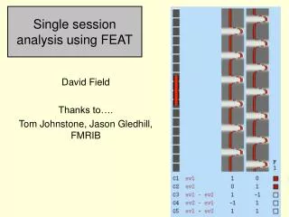
Multi session analysis using FEAT David Field Thanks to…. Tom Johnstone, Jason Gledhill, FMRIB
Overview • Today’s practical session will cover three common group analysis scenarios • Multiple participants do the same single session experiment, and you want the group average activation for one or more contrasts of interest (e.g. words – nonwords) • equivalent to one sample t test versus test value of 0 • Multiple participants are each scanned twice, and you want to know where in the brain the group average activation differs between the two scanning sessions (e.g. before and after a drug) • equivalent to repeated measures t test • Two groups of participants perform the same experimental conditions, and you are interested in where in the brain activation differs between the two groups (e.g. old compared to young) • equivalent to between subjects t test • Today’s lecture will • revisit the outputs of the first level analysis • explain how these outputs are combined to perform a higher level analysis
First level analysis: design matrix EV1 EV2 HRF model
First level analysis: fit model using GLM • For each EV in the design matrix, find the parameter estimate (PE), or beta weight • In the example with 2 EV’s the full model fit for each voxel time course will be • (EV1 time course * PE1) + (EV2 time course * PE2) • note, a PE can be 0 (no contribution of that EV to modelling this voxel time course) • note, a PE can also be negative (the voxel time course dips below its mean value when that EV takes a positive value)
blue: original time course = green: best fitting model (best linear combination of EV’s) + red: residuals (Error)
Looking at EV’s and PE’s using fslview Auditory stimulation periods Visual stimulation periods
Let’s take a look at an original voxel time course, the full model fit, and the fits of individual EV’s using fslview…
First level analysis: voxelwise • The GLM is used to fit the same design matrix independently to every voxel times series in the data set • spatial structure in the data is ignored by the fitting procedure • This results in a PE at every voxel for each EV in the design matrix • effectively, a separate 3D image volume of PE’s for each EV in the original design matrix you can find on the hard disk after running the “stats” tab in FEAT
COPE images • COPE = linear combination of parameter estimates (PE’s) • Also called a contrast, shown as C1, C2 etc on design matrix • The simplest COPE is identical to a single PE image • C1 is 1*PE1 + 0*PE2 etc
COPE images • You can also combine PE’s into COPES in more interesting ways • C3 is 1*PE1 + -1 *PE2 • C3 has high values for voxels where there is a large positive difference between the vis PE and the aud PE C3 1 0 -1 0
VARCOPE images and t statistic images • Each COPE image FEAT creates is accompanied by a VARCOPE image • similar to standard error • based on the residuals • t statistic image = COPE / VARCOPE • Effect size estimate / uncertainty about the estimate • t statistics can be converted to p values or z statistic images • Higher level analysis is similar to first level analysis, but time points are replaced by participants or sessions
Higher level analysis • If two or more participants perform the same experiment, the first level analysis will produce a set of PE and COPE volumes for both subjects separately • how can these be combined these into a group analysis? • The simplest experiments seek brain areas where all the subjects in the group have high values on a contrast • It might help to take a look at the PE / COPE images from some individual participants using fslview….. • finger tapping experiment (motor cortex localiser)
Higher level analysis • You could calculate a voxelwise mean of PE1 from participant1 and PE1 from participant 2 • if both participants have been successfully registered to the MNI template image this strategy would work • but FSL does something more sophisticated, using exactly the same computational apparatus (design matrix plus GLM) that was used at the first level
How FSL performs higher level analysis • FSL carries forward a number of types of images from the lower level to the 2nd level • COPE images • VARCOPES (voxelwise estimates of the standard error of the COPES) • (COPE / VARCOPE produces level 1 t statistic image) • tDOF (images containing the effective degrees of freedom for the lower level time course analysis, taking into account autocorrelation structure of the time course) • Carrying the extra information about uncertainty of estimates and their DOF forward to the higher level leads to a more accurate analysis than just averaging across COPES
Concatenation • First level analysis is performed on 4D images • X, Y, Z, time • Voxel time series of image intensity values • Group analysis is also performed on 4D images • X, Y, Z, participant • Voxel participant-series of effect sizes • Voxel participant-series of standard errors • FSL begins group analysis by concatenating the first level COPES and VARCOPES to produce 4D images • A second level design matrix is fitted using the GLM
Data series at a second level voxel Participant 1 Effect size
Data series at a second level voxel Participant 1 Within participant variance
Data series at a second level voxel Participant 6 Participant 5 Participant 4 Participant 3 Participant 2 Participant 1 Also within subject variance (not shown)
Fixed effects analysis at one voxel Calculate mean effect size across participants (red line)
Fixed effects analysis at one voxel The variance (error term) is the mean of the separate within subject variances
Fixed effects analysis • Conceptually very simple • Many early FMRI publications used this method • It is equivalent to treating all the participants as one very long scan session from a single person • You could concatenate the raw 4D time series data from individual subjects into one series and run one (very large) first level analysis that would be equivalent to a fixed effects group level analysis
Fixed effects analysis • Fixed effects group analysis has fallen out of favour with journal article reviewers • This is because from a statisticians point of view it asks what the mean activation is at each voxel for the exact group of subjects who performed the experiment • it does not take into account the fact that the group were actually a (random?) sample from a population • therefore, you can’t infer that your group results reflect the population • how likely is it that you’d get the same results if you repeated the experiment with a different set of participants rather than the same set? • But it is still commonly used when one participant has performed multiple sessions of the same experiment, and you want to average across the sessions
Random effects analysis • Does the population activate on average? between participant distribution used for random effects within participant variance between participant standard deviation
Random effects analysis • Does the population activate on average? The error term produced by averaging the 6 small distributions is usually smaller than using the between subjects variance as the error term. Therefore, fixed effects analysis is more sensitive to activation (bigger t values) than random effects, but gives less ability to generalize results.
Mixed effects analysis (FSL) • If you want the higher level error term to be made up only of between subjects variance, and to use only the COPE images from level 1, use ordinary least squares estimation (OLS) in FEAT • If you want FSL to also make use of VARCOPE and effective DOF images from level 1, choose FLAME • makes use of first level fixed effects variance as well as the random effects variance in constructing the error term • DOF are also carried forward from level 1 • group activation could be more or less than using OLS, it depends…should be more accurate • outlier deweighting • a way of reducing the effective between subjects error term in the presence of outliers • also reduces impact of outlier on mean • Assumes the sample is drawn from 2 populations, a typical one and an outlier population • For each participant at each voxel estimates the probability that the data point is an outlier, and weights it accordingly
Higher level design matrices in FSL • In a first level design matrix time runs from top to bottom • In a higher level design matrix each participant has one row, and the actual top to bottom ordering has no influence on the model fit • The first column is a number that specifies group membership (will be 1 for all participants if they are all sampled from one population and all did the same experiment) • Other columns are EV’s • A set of contrasts across the bottom • By default the full design matrix is applied to all first level COPE images • results in one 4D concatenation file and one higher level analysis for every lower level COPE image (contrast)
Single group average (one sample t test) EV1 has a value of 1 for each participant, so they are all weighted equally when searching for voxels that are active at the group level. Produces higher level PE1 images This means we consider all our participants to be from the same population. FLAME will estimate only one random effects error term. (Or you could choose fixed effects with same design matrix) Contrast 1 will be applied to all the first level COPE images. If you have lower level COPEs “visual”, “auditory”, and “auditory – visual” then this contrast results in 3 separate group average activation images. Produces higher level COPE1 image * 3
Single group average with covariate EV2 is high for people with slow rtm. Covariates should be orthogonalised wrt the group mean EV1 (demeaned). Produces higher level PE2 images Contrast 2 will locate voxels that are relatively more active in people with slow rtm and less active in people with fast rtm. Produces higher level COPE2 images. A contrast of 0 -1 would locate brain regions that are more active in people with quick reactions and less active in people with slow reactions.
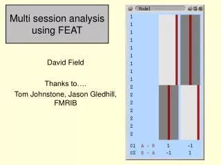
Two samples (unpaired t test) EV1 has a value of 1 for participants 1-9 Participants are sampled from two populations with different variance (e.g. controls and patients). FEAT will estimate two separate random effects error terms. Note unequal group sizes OK. EV1 has a value of 0 for participants 10-16 So, in effect, EV1 models the group mean activation for group 1 (controls). Higher level PE1 images
Two samples (unpaired t test) Subtract image PE1 from image PE2 to produce COPE2, in which voxels with positive values are more active in patients than controls Subtract image PE2 from image PE1 to produce COPE1, in which voxels with positive values are more active in controls than in patients
Paired samples t test • Scan the same participants twice, e.g. memory performance paradigm with and without a drug • Calculate the difference between time 1 scan and time 2 scan at each voxel, for each participant. • The variance in the data due to differences in mean activation level between participants is not relevant if you are interested in the time 1 vs 2 difference • FEAT deals with this by passing the data up to level 2 with between subjects differences, but this source of variation is removed using “nuisance regressors”
Paired samples t test first level COPES from drug condition All participants assigned to the same random effects grouping first level COPES from no-drug condition EV1 has a value of 1 for scans in the “drug” condition and -1 for scans in the “no-drug” condition. Image PE1 will have high values for voxels that are more active in “drug” than in “no drug”
Paired samples t test EV2 has a value of 1 for each of the lower level COPEs from participant 1 and 0 elsewhere. Together with EV’s 3-9 it will model out variation due to between subject (not between condition) differences.
Important note • Any higher level analysis is only as good as the registration of individual participants to the template image…. • If registration is not good then the anatomical correspondence between two participants is poor • functional correspondence cannot be assessed • Registration is more problematic with patient groups and elderly • CHECK YOUR REGISTRATION RESULTS
Cluster size based thresholding • Intuitively, if a voxel with a Z statistic of 1.96 for a particular COPE is surrounded by other voxels with very low Z values this looks suspicious • unless you are looking for a very small brain area • Consider a voxel with a Z statistic of 1.96 is surrounded by many other voxels with similar Z values, forming a large blob • Intuitively, for such a voxel the Z of 1.96 (p = 0.05) is an overestimate of the probability of the model fit to this voxel being a result of random, stimulus unrelated, fluctuation in the time course • The p value we want to calculate is the probability of obtaining one or more clusters of this size or larger under a suitable null hypothesis • “one or more” gives us control over the multiple comparisons problem by setting the family wise error rate • p value will be low for big clusters • p value will be high for small clusters
Comparison of voxel (“height based”) thresholding and cluster thresholding space Significant Voxels No significant Voxels is the height threshold, e.g. 0.001 applied voxelwise (will be Z = about 3)
Comparison of voxel (“height based”) thresholding and cluster thresholding space Cluster significant Cluster not significant k k K is the probability of the image containing 1 or more blobs with k or more voxels (and you can control is at 0.05) The cluster size, in voxels, that corresponds to a particular value of K depends upon the initial value of height threshold used to define the number of clusters in the image and their size It is usual to set height quite low when using cluster level thresholding, but this arbitrary choice will influence the outcome
Dependency of number of clusters on choice of height threshold The number and size of clusters also depends upon the amount of smoothing that took place in preprocessing
Nyquist frequency is important to know about • Half the sampling rate (e.g. TR 2 sec is 0.5 Hz, so Nyquist is 0.25 hz, or 4 seconds) • No signal higher frequency than Nyquist can be present in the data (important for experimental design) • But such signal could appear as an aliasing artefact at a lower frequency