Multiple Regression

1. MultipleRegression

2. Multiple Regression • Consider situations involving two or more independent variables. • This subject area, called multiple regressionanalysis, enables us to consider more factors and thus obtain better estimates than are possible with simple linear regression.

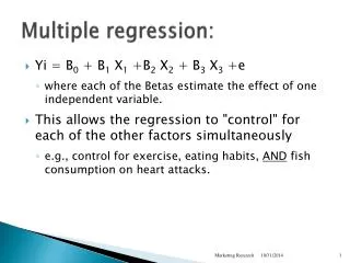
3. Multiple Regression Model • Multiple Regression Model The equation that describes how the dependent variable y is related to the independent variables x1, x2, . . . xp and an error term is: y = b0 + b1x1 + b2x2 +. . . + bpxp + e where: b0, b1, b2, . . . , bp are the parameters, and e is a random variable called the error term

4. Multiple Regression Equation • Multiple Regression Equation The equation that describes how the mean value of y is related to x1, x2, . . . xp is: E(y) = 0 + 1x1 + 2x2 + . . . + pxp

5. ^ y = b0 + b1x1 + b2x2 + . . . + bpxp Estimated Multiple Regression Equation • Estimated Multiple Regression Equation A simple random sample is used to compute sample statistics b0, b1, b2, . . . , bp that are used as the point estimators of the parameters b0, b1, b2, . . . , bp.

6. Sample Data: x1 x2 . . . xp y . . . . . . . . Estimated Multiple Regression Equation Sample statistics are b0, b1, b2, . . . , bp Estimation Process Multiple Regression Model E(y) = 0+ 1x1 + 2x2 +. . .+ pxp + e Multiple Regression Equation E(y) = 0 + 1x1 + 2x2 +. . .+ pxp Unknown parameters are b0, b1, b2, . . . , bp b0, b1, b2, . . . , bp provide estimates of b0, b1, b2, . . . , bp

7. Least Squares Method • Least Squares Criterion • Computation of Coefficient Values The formulas for the regression coefficients b0, b1, b2, . . . bp involve the use of matrix algebra. We will rely on computer software packages to perform the calculations.

8. Multiple Regression Model • Example: Programmer Salary Survey A software firm collected data for a sample of 20 computer programmers. A suggestion was made that regression analysis could be used to determine if salary was related to the years of experience and the score on the firm’s programmer aptitude test. The years of experience, score on the aptitude test test, and corresponding annual salary ($1000s) for a sample of 20 programmers is shown on the next slide.

9. Multiple Regression Model Test Score Exper. (Yrs.) Exper. (Yrs.) Salary ($000s) Salary ($000s) Test Score 4 7 1 5 8 10 0 1 6 6 78 100 86 82 86 84 75 80 83 91 9 2 10 5 6 8 4 6 3 3 88 73 75 81 74 87 79 94 70 89 38.0 26.6 36.2 31.6 29.0 34.0 30.1 33.9 28.2 30.0 24.0 43.0 23.7 34.3 35.8 38.0 22.2 23.1 30.0 33.0

10. Multiple Regression Model Suppose we believe that salary (y) is related to the years of experience (x1) and the score on the programmer aptitude test (x2) by the following regression model: y = 0 + 1x1 + 2x2 +  where y = annual salary ($000) x1 = years of experience x2 = score on programmer aptitude test

11. Solving for the Estimates of 0, 1, 2 Least Squares Output Input Data x1x2y 4 78 24 7 100 43 . . . . . . 3 89 30 Computer Package for Solving Multiple Regression Problems b0 = b1 = b2 = R2 = etc.

12. Solving for the Estimates of 0, 1, 2 • Excel’s Regression Equation Output Note: Columns F-I are not shown.

13. Estimated Regression Equation SALARY = 3.174 + 1.404(EXPER) + 0.251(SCORE) Note: Predicted salary will be in thousands of dollars.

14. Interpreting the Coefficients In multiple regression analysis, we interpret each regression coefficient as follows: bi represents an estimate of the change in y corresponding to a 1-unit increase in xi when all other independent variables are held constant.

15. Interpreting the Coefficients b1 = 1.404 Salary is expected to increase by $1,404 for each additional year of experience (when the variable score on programmer attitude test is held constant).

16. Interpreting the Coefficients b2 = 0.251 Salary is expected to increase by $251 for each additional point scored on the programmer aptitude test (when the variable years of experience is held constant).

17. Multiple Coefficient of Determination • Relationship Among SST, SSR, SSE SST = SSR + SSE + = where: SST = total sum of squares SSR = sum of squares due to regression SSE = sum of squares due to error

18. Multiple Coefficient of Determination R2 = SSR/SST R2 = 500.3285/599.7855 = .83418

19. Adjusted Multiple Coefficient of Determination • Adding independent variables, even ones that are not statistically significant, causes the prediction errors to become smaller, thus reducing the sum of squares due to error, SSE. • Because SSR = SST – SSE, when SSE becomes smaller, SSR becomes larger, causing R2 = SSR/SST to increase. • The adjusted multiple coefficient of determination compensates for the number of independent variables in the model.

20. Adjusted Multiple Coefficient of Determination

21. Testing for Significance: t Test A separate t test is conducted for each of the independent variables in the model. We refer to each of these t tests as a test for individual significance.

22. Testing for Significance: t Test Hypotheses Test Statistics Rejection Rule Reject H0 if p-value <a or if t< -tor t>twhere t is based on a t distribution with n - p - 1 degrees of freedom.

23. t Test for Significance of Individual Parameters Hypotheses Rejection Rule • For  = .05 and d.f. = 17, t.025 = 2.11 • Reject H0 if p-value < .05, or • if t< -2.11 or t> 2.11

24. t Test for Significance of Individual Parameters • Excel’s Regression Equation Output Note: Columns F-I are not shown. t statistic and p-value used to test for the individual significance of “Experience”

25. t Test for Significance of Individual Parameters • Excel’s Regression Equation Output Note: Columns F-I are not shown. t statistic and p-value used to test for the individual significance of “Test Score”

26. t Test for Significance of Individual Parameters Test Statistics Conclusions • Reject bothH0: 1 = 0 and H0: 2 = 0. • Estimated coefficients on both • independent variables are significant.

27. Using the Estimated Regression Equationfor Estimation and Prediction The procedures for estimating the mean value of y and predicting an individual value of y in multiple regression are similar to those in simple regression. We substitute the given values of x1, x2, . . . , xp into the estimated regression equation and use the corresponding value of y as the point estimate.

28. The formulas required to develop interval estimates for the mean value of y and for an individual value of y are beyond the scope of the course. ^ Using the Estimated Regression Equationfor Estimation and Prediction Software packages for multiple regression will often provide these interval estimates.

29. Categorical Independent Variables In many situations we must work with categorical independent variablessuch as gender (male, female), method of payment (cash, check, credit card), etc. For example, x2 might represent gender where x2 = 0 indicates male and x2 = 1 indicates female. In this case, x2 is a dummy or indicator variable.

30. Categorical Independent Variables • Example: Programmer Salary Survey The years of experience, the score on the programmer aptitude test, whether the individual has a relevant graduate degree, and the annual salary ($000) for each of the sampled 20 programmers are shown on the next slide. As an extension of the problem involving the computer programmer salary survey, suppose that management also believes that the annual salary is related to whether the individual has a graduate degree in computer science or information systems.

31. Categorical Independent Variables Exper. (Yrs.) Test Score Salary ($000s) Exper. (Yrs.) Test Score Salary ($000s) Degr. Degr. 4 7 1 5 8 10 0 1 6 6 78 100 86 82 86 84 75 80 83 91 No Yes No Yes Yes Yes No No No Yes 9 2 10 5 6 8 4 6 3 3 88 73 75 81 74 87 79 94 70 89 Yes No Yes No No Yes No Yes No No 38.0 26.6 36.2 31.6 29.0 34.0 30.1 33.9 28.2 30.0 24.0 43.0 23.7 34.3 35.8 38.0 22.2 23.1 30.0 33.0

32. ^ y = b0 + b1x1 +b2x2 + b3x3 where: y = annual salary ($1000) x1 = years of experience x2 = score on programmer aptitude test x3 = 0 if individual does not have a graduate degree 1 if individual does have a graduate degree ^ Estimated Regression Equation x3 is a dummy variable

33. Categorical Independent Variables • Excel’s Regression Statistics Previously, R Square = .8342 Previously, Adjusted R Square = .815 (essentially no improvement)

34. Categorical Independent Variables • Excel’s Regression Equation Output Note: Columns F-I are not shown. Not significant

35. Categorical Independent Variables • Excel’s Regression Equation Output Note: Columns C-E are hidden.

36. Modeling Curvilinear Relationships • Example: Sales of Laboratory Scales A manufacturer of laboratory scales wants to investigate the relationship between the length of employment of their salespeople and the number of scales sold. The table on the next slide gives the number of months each salesperson has been employed by the firm (x) and the number of scales sold (y) by 15 randomly selected salespersons.

37. Modeling Curvilinear Relationships • Example: Sales of Laboratory Scales Months Months Sales Sales 189 235 83 112 67 325 189 40 51 9 12 6 56 19 275 296 317 376 162 150 367 308 41 106 76 104 22 12 85 111

38. Modeling Curvilinear Relationships Excel’s Chart tools can be used to develop a scatter diagram and fit a straight line to bivariate data. The estimated regression equation and the coefficient of determination for simple linear regression can also be developed. The results of using Excel’s Chart tools to fit a line to the data are shown on the next slide.

39. Modeling Curvilinear Relationships • Chart Tools Output

40. Modeling Curvilinear Relationships The scatter diagram indicates a possible curvilinear relationship between the length of time employed and the number of scales sold. So, we develop a multiple regression model with two independent variables: x and x2. y = b0+ b1x+b2x2+ e This model is often referred to as a second-order polynomial or a quadratic model.

41. Modeling Curvilinear Relationships Excel’s Chart tools can be used to fit a polynomial curve to the data. (Dialog box is on next slide.) To get the dialog box, position the mouse pointer over any data point in the scatter diagram and right-click. The estimated multiple regression equation and multiple coefficient of determination for this second- order model are also obtained.

42. Modeling Curvilinear Relationships • Chart Tools Output

43. Modeling Curvilinear Relationships • Second Independent Variable (MonthSq) Added MonthsSq Months Months MonthsSq Sales Sales 189 235 83 112 67 325 189 40 51 9 12 6 56 19 1600 2601 81 144 36 3136 361 275 296 317 376 162 150 367 308 41 106 76 104 22 12 85 111 1681 11236 5776 10816 484 144 7225 12321

44. Modeling Curvilinear Relationships • Excel’s Regression Tool Output We should be pleased with the fit provided by the estimated multiple regression equation.

45. Modeling Curvilinear Relationships • Excel’s Regression Tool Output The overall model is significant (p-value for the F test is 8.75E-07).

46. Modeling Curvilinear Relationships • Excel’s Regression Tool Output We can conclude that adding MonthsSq to the model is significant.