
Sampling and Aliasing
E N D
Presentation Transcript
Sampling and Aliasing Gilad Lerman Math 5467 (stealing slides from Gonzalez & Woods, and Efros)
The Sampling Theorem Theorem: If f is in L1() & supported on [-B0, B0], then Recall Proof: We view as (2B0)-periodic function with coefficients: At last, find f using IFT and using FS of
More on the Sampling Theorem Frequency band: Time: Note: Theorem holds for B>B0. Indeed, then If B<B0, the above equation is not true for all
Sampling Theorem (meaning) • Interpretation: If a function f(t) contains no frequencies higher than W cps, it is completely determined by giving its ordinates at a series of points spaced 1/(2W) seconds apart • Remark: For L1 function a freq. = W is fine but for more general functions we need > W…
Simple Example (not L1) Assume a cosine (it is not L1() but will be instrumental) Freq: a (“& -a”), Freq Band: =[-a,a], Time: 1/(2a) Here one needs B>B0 (B=B0 doesn’t work) Example: for all 3 functions freq: 0.5, time: 1 The sampled function has different aliases…
Aliasing • If the sampling condition is not satisfied, frequencies will overlap (high freq → low freq) • The reconstructed signal is said to be an alias of the original signal
Input signal: Matlab output: x = 0:.05:5; imagesc(sin((2.^x).*x)) Example: Increased Frequency Related Image: Picket fence receding Into the distance will produce aliasing…
Good and Bad Sampling • Good sampling: • Sample often or, • Sample wisely • Bad sampling: • see aliasing in action!
Even worse for synthetic images Slide by Steve Seitz
Really bad in video Slide by Paul Heckbert
Moiré pattern • Definition: Interference pattern created, e.g., when two grids are overlaid at an angle, or when they have slightly different mesh sizes. • In images produced e.g., when scanning a halftone picture or due to undersampling a fine regular pattern.
Moiré pattern due to undersampling Original image downsampled image
Antialiasing • What can be done? Sampling rate ≥ 2 * max frequency in the image • Raise sampling rate by oversampling • Sample at k times the resolution • continuous signal: easy • discrete signal: need to interpolate • 2. Lower the max frequency by prefiltering • Smooth the signal enough • Works on discrete signals • 3. Improve sampling quality with better sampling • Nyquist is best case! • Stratified sampling • Importance sampling • Relies on domain knowledge
Gaussian pre-filtering G 1/8 G 1/4 Gaussian 1/2 • Solution: filter the image, then subsample • Filter size should double for each ½ size reduction.
Subsampling with Gaussian pre-filtering Gaussian 1/2 G 1/4 G 1/8
Compare with... 1/2 1/4 (2x zoom) 1/8 (4x zoom)
Rethinking of the Cooley-Tukey FFT • Step 1(top to bottom): Create two subsampled signals (even and odd coordinates) • Note that the two subsampled signals are associated with half bands in the frequency domain (Shannon) • Step 2 (bottom-up): Combine the two signals by the formulas: • Interpretation: combining the two half bands in the right way (in frequency domain) to exactly recover the signal