Threats to validity in observational studies Jay S. Kaufman, PhD

1. Threats to validity in observational studies Jay S. Kaufman, PhD McGill University, Montreal QC 25 February 2016 11:05 AM – 11:45 AM National Academy of Sciences 2101 Constitution Ave NW, Washington, DC 20418 USA

2. Statistical models are used to estimate relationships between variables in observational data sets. Y Y β1 β0 0 1 X X

3. Three main inferential targets of these models: 1) Real world in the present 2) Real world in the future 3) Hypothetical world in the future The inferential target determines the adjustment strategy. Most people here are interested in 3) surveillance, descriptive study clinical prediction model causal inference, etiologic study

4. If you are trying to estimate the causal effect of a treatment, your job is to PREDICT what would happen in the FUTURE if you did thing A compared to what would happen if you did thing B. To do this from observational data, you must often adjust statistically for factors that are associated with the treatment and the outcome. You observe: Pr(Y|X=x) You want to know: Pr(Y|SET[X=x]) This is the intervention you want to know about, but unfortunately you don’t really get to “SET” anything.

5. The adjustment tradition in statistics exists to link these two quantities: Z Pr(Y|X=x)  Pr(Y|SET[X=x]) X Y BUT! ΣPr(Y|X=x, Z=z)Pr(Z=z) = Pr(Y|SET[X=x])

6. Read: Pr(Y|SET[X=x]) as: Pr(Y|SET[X=x1]) versus Pr(Y|SET[X=x2]) x1 and x2 are the levels at which you intervene to set the treatment; contrast is usually a difference or ratio. Causal inference from passively observed data requires not just structural identification, but also: positivity (there are sufficient data available on the treatment and outcome in the range of interest) consistency (the way that people came to be treated in the data set is comparable to the way that you plan to treat them in your intervention) correct specification of statistical models

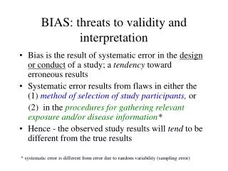
7. Three main structural threats to validity: Confounding Bias Selection Bias Information Bias Z X Y Z X Y X* Y* U X Y

8. If you didn’t get to Z by one pathway, you are more likely to have gotten there via the other pathway: A Z B π A B A Z π A B | Z B Hernán MA, Hernández-Díaz S, Robins JM. A structural approach to selection bias. Epidemiology 2004 Sep;15(5):615-25.

9. If you didn’t get to Z by one pathway, you are more likely to have gotten there via the other pathway: smoking Clinical Diagnosis genetic mutation smoking Clinical Diagnosis genetic mutation Cole SR, et al. Illustrating bias due to conditioning on a collider. Int J Epidemiol. 2010 Apr;39(2):417-20.

10. Banack HR, Kaufman JS. The "obesity paradox" explained. Epidemiology 2013; 24: 461-2. Banack HR, Kaufman JS. The obesity paradox: understanding the effect of obesity on mortality among individuals with CVD. Prev Med 2014; 62: 96-102. Banack HR, Kaufman JS. Does selection bias explain the obesity paradox among individuals with cardiovascular disease? Ann Epidemiol2015 May;25(5):342-9. Lajous M, Banack HR, Kaufman JS, HernánMA. Should patients with chronic disease be told to gain weight? Am J Med 2015;128(4):334-6.

11. Canto et al. JAMA 2011;306(19):2120-2127.

12. 5 major CHD risk factors: Hypertension Smoking Dyslipidemia Diabetes Family hx of CHD 25% of original cohort

13. Pre-hospital MI mortality is a collider, making risk factors associated with every U among those selected (S). Effect estimators will thus be biased if any U is not controlled. So, in contrast to previous descriptions, bias will exist even if MI hospitalization is not confounded. U Pre-Hosp Mortality S MI Hospital- ization Post Hosp Mortality Risk Factors Flanders WD, et al. A Nearly Unavoidable Mechanism for Collider Bias with Index-Event Studies. Epidemiology 2014 Sep;25(5):762-4.

14. Therefore, selection bias results in this • example from: • Recruiting MI hospitalized patients into the study when • there are common unmeasured causes of MI • hospitalization and mortality • Removal of the frailest people via pre-hospital mortality • (maybe around 30%?) • Removal of 75% of the hospitalized cohort with prior • CVD diagnosis or transfer within 30 days • This is easily enough to produce a paradoxical reverse • association in which the risk factors erroneously appear • protective, even if there is no individual whose risk is • lowered by the presence of one of these factors.

15. Some additional selection bias structures: Treatment Death Censoring Symptoms U Unmeasured variable U represents underlying disease severity, and those with more severe disease have a greater risk of death. Patients with more severe disease are more likely to be censored because they are unwell. Patients receiving treatment are at a greater risk of experiencing side effects, which also lead to drop-out.

16. Some additional selection bias structures: Treatment Symptoms U Censoring Death In this variation of the previous structure, treatment and underlying severity both affect symptoms, which in turn affects drop-out. The censoring as a function of symptoms, which is affected by both treatment and U, creates the same conditional dependency.

17. Other mechanisms of selection bias: • Differential loss to follow-up, also known as “informative censoring” • Missing data bias, nonresponse bias: Censoring can represent missing data on the outcome for any reason, not just as a result of loss to follow up. • Healthy worker bias: Effect of an occupational chemical in a factory. Unmeasured illness is predictive of death and of missing work, but only subjects at work are recruited. • Self-selection bias, volunteer bias • Selection affected by treatment received before study entry (left-truncation)

18. Survival Produces an Unavoidable Selection Bias: Start out with a randomized trial so that all covariates are balanced at time 0. Once events occur, if you condition your estimate on having survived to the next time point, every other cause of disease must now be correlated with exposure. Genetic Variant Genetic Variant Death Death Treat ment Treat ment = ? = 0 time 2 time 1 Flanders WD, Klein M. Properties of 2 counterfactual effect definitions of a point exposure. Epidemiology2007; 18(4):453-60.

19. This is exactly why the HAZARD RATIO (the parameter estimated by a Cox Proportional Hazards Model) should not be used (unless the outcome is rare): The hazard of death at time 1 is the probability of dying at time 1. But the hazard at time 2 is the probability of dying at time 2 among those who survived past time 1: Treated survivors of time 1 differ in their distribution of U compared to untreated survivors of time 1, making this conditional measure confounded by U in a way that a marginal measure is not. This concern applies to both observational studies and randomized experiments. Treatment Y1 Y2 U

20. Why do we continue to base inference on so many confusing studies that use highly selected samples, such as diagnosed patients? There is a simple design concept to avoid this mess…

21. An important step in eliminating “obesity paradox” and similar selection biases is just to ensure that the start of exposure and the start of follow-up coincide. That is exactly how we analyze randomized clinical trials: Nobody would ever propose an RCT that would select individuals free of disease 5 years after randomization and then compare the disease incidence between arms only from that point forward.

22. A simple rule of ensuring that the start of follow-up and initiation of treatment coincide is natural in RCTs, but often overlooked when analyzing observational studies. For example, widespread confusion about the cardiovascular effects of hormone therapy resulted from observational analyses that effectively ignored the first few years of follow-up by comparing prevalent users versus never users. Admittedly, this rule is hard to apply to exposures like obesity that lack a clear onset, but should be very clear for medical and pharmacological interventions. Hernán MA, Robins JM. Observational Studies Analyzed Like Randomized Experiments: Best of Both Worlds. Epidemiology 2008;19:789-92.

23. Then estimate risk of outcome at each follow-up time, without conditioning on survival up to that point (just comparing to the baseline denominator) Causal effect estimate is the difference between covariate-standardized survival curves at time t Hernán MA, The hazards of hazard ratios. Epidemiology 2010;21(1):13-5.

24. To the extent that confounding and selection bias are due to measured covariates C, these can be handled by inverse weighting (IPTW, IPCW) This is especially convenient for longitudinal data in which the confounder C may be effected by previous treatment Xt and may in turn influence the next dose of treatment Xt+1. It is also helpful in the longitudinal setting where the remaining cohort at each time t becomes increasing selected. Reweighting the cohort by measured characteristics allows remaining subjects to proxy for the ones that are missing. C X Y Z C X Y

25. Summary: Models are used to parameterize associations between treatment and response variables. Often, we want to interpret these associations causally (i.e. predicting the change in Y that would occur under some specific intervention on X). The validity of this causal interpretation is threatened by systematic and random errors. The systematic errors include confounding bias, which get a lot of attention in training and practice. Information bias and selection bias are other important sources of systematic error, and should be considered more frequently and thoughtfully in design and analysis.