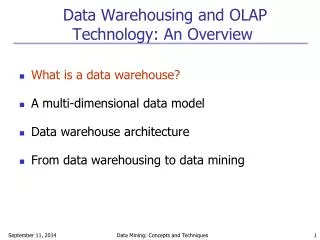
Data Warehousing and OLAP Technology for Data Mining
Data Warehousing and OLAP Technology for Data Mining. What is a data warehouse? A multi-dimensional data model Data warehouse architecture Data warehouse implementation Further development of data cube technology From data warehousing to data mining. What is Data Warehouse?.

Data Warehousing and OLAP Technology for Data Mining
E N D
Presentation Transcript
Data Warehousing and OLAP Technology for Data Mining • What is a data warehouse? • A multi-dimensional data model • Data warehouse architecture • Data warehouse implementation • Further development of data cube technology • From data warehousing to data mining
What is Data Warehouse? • Defined in many different ways • A decision support database that is maintained separately from the organization’s operational database • Support information processing by providing a solid platform of consolidated, historical data for analysis. • “A data warehouse is asubject-oriented, integrated, time-variant, and nonvolatilecollection of data in support of management’s decision-making process.”—W. H. Inmon
Data Warehouse—Subject-Oriented • Organized around major subjects, such as customer, product, sales. • Focusing on the modeling and analysis of data for decision makers, not on daily operations or transaction processing. • Provide a simple and concise view around particular subject issues by excluding data that are not useful in the decision support process.
Data Warehouse—Integrated • Constructed by integrating multiple, heterogeneous data sources • relational databases, flat files, on-line transaction records • Data cleaning and data integration techniques are applied. • Ensure consistency in naming conventions, encoding structures, attribute measures, etc. among different data sources • When data is moved to the warehouse, it is converted.
Data Warehouse—Time Variant • The time horizon for the data warehouse is significantly longer than that of operational systems. • Operational database: current value data. • Data warehouse data: provide information from a historical perspective (e.g., past 5-10 years) • Every key structure in the data warehouse • Contains an element of time, explicitly or implicitly • But the key of operational data may or may not contain “time element”.
Data Warehouse—Non-Volatile • A physically separate store of data transformed from the operational environment. • Operational update of data does not occur in the data warehouse environment. • Does not require transaction processing, recovery, and concurrency control mechanisms • Requires only two operations in data accessing: • initial loading of data and access of data.
Data Warehouse vs. Heterogeneous DBMS • Many Organizations may collect diverse kinds of Heterogeneous Dbases such as Multiple, Autonomous and Distributed Information sources • Integration of these are must for easy and efficient access • Traditional heterogeneous DB integration: • Build wrappers/mediators on top of heterogeneous databases • Query driven approach • When a query is posed to a client site, a meta-dictionary is used to translate the query into queries appropriate for individual heterogeneous sites involved, and the results are integrated into a global answer set • Complex information filtering, compete for resources • Data warehouse: update-driven, high performance • Information from heterogeneous sources is integrated in advance and stored in warehouses for direct query and analysis
Data Warehouse vs. Operational DBMS • OLTP (on-line transaction processing) • Major task of traditional relational DBMS • Day-to-day operations: purchasing, inventory, banking, manufacturing, payroll, registration, accounting, etc. • OLAP (on-line analytical processing) • Major task of data warehouse system • Data analysis and decision making • Distinct features (OLTP vs. OLAP): • User and system orientation: customer vs. market • Data contents: current, detailed vs. historical, consolidated • View: current, local vs. evolutionary, integrated • Access patterns: update vs. read-only but complex queries
Why Separate Data Warehouse? • We know that Operational Databases store huge amounts of data • Why not perform ILAP directly on such Dbases instead of spending additional time and resources to construct a separate data warehouse? • The Major reason is…
Why Separate Data Warehouse? • High performance for both systems • DBMS— tuned for OLTP: access methods, indexing, concurrency control, recovery • Warehouse—tuned for OLAP: complex OLAP queries, multidimensional view, consolidation. • Different functions and different data: • missing data: Decision Support requires historical data which operational DBs do not typically maintain • data consolidation: DS requires consolidation (aggregation, summarization) of data from heterogeneous sources • data quality: different sources typically use inconsistent data representations, codes and formats which have to be reconciled
Data Warehousing and OLAP Technology for Data Mining • What is a data warehouse? • A multi-dimensional data model • Data warehouse architecture • Data warehouse implementation • Further development of data cube technology • From data warehousing to data mining
Data Warehousing and OLAP Technology for Data Mining • A data warehouse is based on a multi-dimensional data model which views data in the form of a data cube • Data Cube allowed to be modeled multiple dimensions • A data cube, such as sales, allows data to be modeled and viewed in multiple dimensions • Dimension tables, such as item (item_name, brand, type), or time(day, week, month, quarter, year) • Fact table contains measures (such as dollars_sold) and keys to each of the related dimension tables • In data warehousing literature, an n-D base cube is called a base cuboid. The top most 0-D cuboid, which holds the highest-level of summarization, is called the apex cuboid. The lattice of cuboids forms a data cube.
Cube: A Lattice of Cuboids all Highest Level of Summarization 0-D(apex) cuboid time item location supplier 1-D cuboids time,item time,location item,location location,supplier 2-D cuboids time,supplier item,supplier time,location,supplier time,item,location 3-D cuboids item,location,supplier time,item,supplier 4-D(base) cuboid time, item, location, supplier
Conceptual Modeling of Data Warehouses • The most popular data model for a data warehouse is a Multidimensional Model • There are different forms • Star schema • Snowflake schema • Fact constellations schema
Star Schema • This is the most common modeling paradigm • It contains a large central table called fact table , which containing the bulk of data with no redundancy • And it has a set of smaller attendant tables called dimension tables for each dimension
item time item_key item_name brand type supplier_type time_key day day_of_the_week month quarter year location branch Attributes such as location_key street city province_or_street country branch_key branch_name branch_type Example of Star Schema Supplier / Location are redundant Sales Fact Table time_key item_key branch_key location_key units_sold dollars_sold avg_sales Measures
Defining a Star Schema in DMQL define cube sales_star [time, item, branch, location]: dollars_sold = sum(sales_in_dollars), avg(sales_in_dollars), units_sold = count(*) define dimension time as (time_key, day, day_of_week, month, quarter, year) define dimension item as (item_key, item_name, brand, type, supplier_type) define dimension branch as (branch_key, branch_name, branch_type) define dimension location as (location_key, street, city, province_or_state, country)
Snowflake schema • A refinement of star schema where some dimensional hierarchy is normalized into a set of smaller dimension tables, forming a shape similar to snowflake
supplier item time item_key item_name brand type supplier_key supplier_key supplier_type time_key day day_of_the_week month quarter year city location branch city_key city province_or_street country location_key street city_key branch_key branch_name branch_type Example of Snowflake Schema Sales Fact Table time_key item_key branch_key location_key units_sold dollars_sold avg_sales Measures
Defining a Snowflake Schema in DMQL define cube sales_snowflake [time, item, branch, location]: dollars_sold = sum(sales_in_dollars), define dimension time as (time_key, day, day_of_week, month, quarter, year) define dimension item as (item_key, item_name, brand, type, supplier(supplier_key, supplier_type)) define dimension branch as (branch_key, branch_name, branch_type) define dimension location as (location_key, street, city(city_key, province_or_state, country))
Fact constellations • Sophisticated applications may require multiple fact tables to share dimension tables • It can be viewed as a collection of stars, therefore called galaxy schema or fact constellation • Two fact tables : sales and shipping
item time item_key item_name brand type supplier_type time_key day day_of_the_week month quarter year location location_key street city province_or_street country shipper branch shipper_key shipper_name location_key shipper_type branch_key branch_name branch_type Example of Fact Constellation Shipping Fact Table time_key Sales Fact Table item_key time_key shipper_key item_key from_location branch_key to_location location_key dollars_cost units_sold units_shipped dollars_sold avg_sales Measures
Defining a Fact Constellation in DMQL define cube sales [time, item, branch, location]: dollars_sold = sum(sales_in_dollars), avg_sales = avg(sales_in_dollars), units_sold = count(*) define dimension time as (time_key, day, day_of_week, month, quarter, year) define dimension item as (item_key, item_name, brand, type, supplier_type) define dimension branch as (branch_key, branch_name, branch_type) define dimension location as (location_key, street, city, province_or_state, country) define cube shipping [time, item, shipper, from_location, to_location]: dollar_cost = sum(cost_in_dollars), unit_shipped = count(*) define dimension time as time in cube sales define dimension item as item in cube sales define dimension shipper as (shipper_key, shipper_name, location as location in cube sales, shipper_type) define dimension from_location as location in cube sales define dimension to_location as location in cube sales
Data Warehouse vs Data Mart • DWarehouse collects the information about the subjects of the entire organizations • Fact constellation should be used • DMart focuses on selected subjects like department-wide • Star or Snowflake can be used
Multidimensional Data • Sales volume as a function of product, month, and region Dimensions: Product, Location, Time Hierarchical summarization paths Region Industry Region Year Category Country Quarter Product City Month Week Office Day Product Month
Date 2Qtr 1Qtr sum 3Qtr 4Qtr TV Product U.S.A PC VCR sum Canada Country Mexico sum All, All, All A Sample Data Cube Total annual sales of TV in U.S.A.
Data Preprocessing • Data Cleaning • Data Integration and Transformation and • Data Reduction
Why Data Preprocessing? • Data in the real world is dirty • incomplete: lacking attribute values, lacking certain attributes of interest, or containing only aggregate data • noisy: containing errors or outliers • inconsistent: containing discrepancies in codes or names • No quality data, no quality mining results! • Quality decisions must be based on quality data • Data warehouse needs consistent integration of quality data
Multi-Dimensional Measure of Data Quality • A well-accepted multidimensional view: • Accuracy • Completeness • Consistency • Timeliness • Believability • Value added • Interpretability • Accessibility • Broad categories: • intrinsic, contextual, representational, and accessibility.
Major Tasks in Data Preprocessing • Data Cleaning • Fill in missing values, smooth noisy data, identify or remove outliers, and resolve inconsistencies • Data Integration • Integration of multiple databases, data cubes, or files • Data Transformation • Normalization and aggregation • Data Reduction • Obtains reduced representation in volume but produces the same or similar analytical results
Data Cleaning • Data cleaning tasks • Fill in missing values • Identify outliers and smooth out noisy data • Correct inconsistent data
Missing Data • Data is not always available • E.g., many tuples have no recorded value for several attributes, such as customer income in sales data • Missing data may be due to • equipment malfunction • inconsistent with other recorded data and thus deleted • data not entered due to misunderstanding • certain data may not be considered important at the time of entry • not register history or changes of the data • Missing data may need to be inferred.
How to Handle Missing Data? • Ignore the tuple: usually done when class label is missing (assuming the tasks in classification—not effective when the percentage of missing values per attribute varies considerably. • Fill in the missing value manually: tedious + infeasible? • Use a global constant to fill in the missing value: e.g., “unknown”, a new class?! • Use the attribute mean to fill in the missing value • Use the attribute mean for all samples belonging to the same class to fill in the missing value: smarter • Use the most probable value to fill in the missing value: inference-based such as Bayesian formula or decision tree
Noisy Data • Noise: random error or variance in a measured variable • Incorrect attribute values may due to • faulty data collection instruments • data entry problems • data transmission problems • technology limitation • inconsistency in naming convention • Other data problems which requires data cleaning • duplicate records • incomplete data • inconsistent data
How to Handle Noisy Data?/ Smoothing • Binning method( for Data Transformation) • first sort data and partition into (equi-depth) bins • then one can smooth by bin means, smooth by bin median, smooth by bin boundaries, etc. • Clustering • detect and remove outliers • Combined computer and human inspection • detect suspicious values and check by human • Regression • smooth by fitting the data into regression functions
Regression y Y1 y = x + 1 Y1’ x X1
Data Integration • Data integration: • combines data from multiple sources into a coherent store • Schema integration • integrate metadata from different sources • Entity identification problem: identify real world entities from multiple data sources, e.g., A.cust-id B.cust-# • Detecting and resolving data value conflicts • for the same real world entity, attribute values from different sources are different • possible reasons: different representations, different scales, e.g., metric vs. British units
Handling Redundant Data in Data Integration • Redundant data occur often when integration of multiple databases • The same attribute may have different names in different databases • One attribute may be a “derived” attribute in another table, e.g., annual revenue • Redundant data may be able to be detected by correlational analysis • Careful integration of the data from multiple sources may help reduce/avoid redundancies and inconsistencies and improve mining speed and quality
Data Transformation • Smoothing: remove noise from data ( binning, clustering, Regression) • Aggregation: Daily sales data may be aggreagated to so as to compute monthly / yearly • Which is used for analysis • ie summarization or data cube construction • Generalization: low-level data replaced by higher-level data • Street to city/country • Age to like young, middle-age or senior
Data Transformation • Normalization: scaled to fall within a small, specified range • -1.0 to 1.0 or 0.0 to 1.0 • There are three types • Min-Max • Z-score and • Normalization by decimal scaling • Attribute/feature construction • New attributes constructed from the given ones tp help the mining process
Data Transformation: Normalization • min-max normalization • z-score normalization • normalization by decimal scaling Where j is the smallest integer such that Max(| |)<1
Data Reduction Strategies • Warehouse may store terabytes of data: Complex data analysis/mining may take a very long time to run on the complete data set • Data reduction • Obtains a reduced representation of the data set that is much smaller in volume but yet produces the same (or almost the same) analytical results • Data reduction strategies • Data cube aggregation • Dimensionality reduction • Data Compression • Numerosity reduction
Data Cube Aggregation • Minimizing information from Multidimensional analysis of sales
Dimensionality Reduction • Data sets for analysis may contain hundreds of attributes • Many of which may be irrelavant to the mining task or redundant • It reduces the data set size by removing such attributes from it Reduction Techniques • step-wise forward selection – procedure starts with empty set of attributes and the best attribute is added to the set • step-wise backward elimination • combining forward selection and backward elimination • decision-tree induction- Tree constructed with the given data. If Attributes that do not appear in the tree are declared irrelevant
> Example of Decision Tree Induction Initial attribute set: {A1, A2, A3, A4, A5, A6} A4 ? A6? A1? Class 2 Class 2 Class 1 Class 1 Reduced attribute set: {A1, A4, A6}
Data Compression • String compression • There are extensive theories and well-tuned algorithms • Typically lossless • But only limited manipulation is possible without expansion • Audio/video compression • Typically lossy compression, with progressive refinement • Sometimes small fragments of signal can be reconstructed without reconstructing the whole • Time sequence is not audio • Typically short and vary slowly with time