Download
1 / 34
340 likes | 492 Vues
Learn to solve second-order linear DEs and analyze systems like vibrating springs, explore damping effects, and apply diagonalization method. Understand eigenvalues, convergence, equilibrium points, and graphical phase planes.

E N D
ENGG2013 Unit 25Second-order Linear DE Apr, 2011.
Yesterday • First-order DE • Method of separating variable • Method of integrating factor • System of first-order DE • Eigenvalues determine the convergence behaviour near a critical point. • Objectives: • Solve the initial value problem • Given the initial value, find the trajectory • Transient-state analysis of electronic circuits • Understand the system behaviour • Does the system converge? • Stable equilibrium point, unstable equilibrium point. kshum
Linear Second-order DE • Homogeneous • Non-homogeneous kshum
Linear Second-order constant-coeff. DE • Homogeneous • Non-homogeneous kshum
Vibrating spring without damping k x m x’’ x Second-order, autonomouslinear, constant-coefficientand homogeneous m x’’ + k x = 0 • Assumptions: • Spring has negligible weight • No friction • x(t): vertical displacement • Hooke’s law: Force = k x • k is the spring constant, k > 0(the constant k is sometime called the spring modulus.) • Newton’s law: F = m x’’ • m is the mass, m > 0 kshum
Solutions to undamped spring-mass model Normalize by m Direct substitution verifies that andare solutions, e.g. kshum
Natural frequency • Let • We know that cos( t) and sin( t) are both solutions. • is called the natural frequency. • Dimension check: The unit of is Hz = s-1. • The spring constant k has unit kg s-2. • k/m has unit s-2. • Square root of k/m has unit s-1. kshum
Principle of superposition(aka linearity principle) For linear and homogenous differential equation, the linear combination of two solutions is also a solution. For any real numbers a and b, a cos( t) + b cos( t) is a solution to x’’+ 2x=0. kshum
GRAPHICAL METHOD kshum
Graphical illustration of spring-mass model Define the displacement-velocity vector Reduction to system of two first-order differential equations. kshum
Phase plane for the vibrating spring Sample solution The trajectory is a ellipse kshum
Order reduction technique equivalent Second-order DE with constant coefficients is basicallythe same as a system of two first-order DE. kshum
Vibrating spring with damping m x’’ = – k x – d x’ honey Force exerted by the spring Assumption: Magnitude of damping forceis directly proportional to x’. d> 0 Damping due to viscosity Equivalent form Vibrating spring in honey kshum
Phase plane for damped spring Sample solutions Convergenceto the origin kshum
Recall: Diagonalization Definition: an nn matrix M is called diagonalizable if we can find an invertible matrix S, such thatis a diagonal matrix, or equivalently, Example: Diagonalization is useful in decoupling a linear system for instance.
Solution to vibrating spring with damping Characteristic equation Eigenvalues
Solution to vibrating spring with damping Eigenvectors have complex components Two eigenvectors are notscalar multiple of each other, because the two eigenvalues aredistinct . Hence inverse exists. Concatenate Diagonalize
Solution to vibrating spring with damping Substitute by the diagonalized matrix Change of variables An uncoupled system
Solution to vibrating spring with damping Solve the uncoupled system K1 and K2 are constants Substitute back (C1, C1, a and b are constants)
A general strategy for linear system Decouple(Diagonalization) Solve each subsystem separately Solved Piece themtogether Linear system
2nd-order constant-coeff. DE • Homogeneous • b and c are constants. • Non-homogeneous • b and c are constants. • f(t) is a function of independent variable t. kshum
The homogeneous case • Idea: try a function in the form ektas a solution. • k is some constant. • Substitute ektinto x’’+bx’+cx=0 and try to solve for the constant k. • Apply the superposition principle: any linear combination of solutions is also a solution. kshum
Examples • Solve x’’+3x’+2x=0. • Solve x’’–4x’+4x=0. • Solve x’’+9x= 0. General solution: x(t) = c1 e–2t+ c2e–t General solution: x(t) = c1 e2t+ c2 t e2t General solution: x(t) = c1 e3i t+ c2 e-3i t = d1 sin(t)+ d2 cos(t) kshum
Summary of the three cases Differential equation Characteristic equation kshum
The non-homogeneous case • Property: If x1(t) and x2(t) are two solutions to then their difference x1(t) – x2(t) is a solution to the homogeneous counterpart kshum
Consequence • Suppose that xp(t) is some solution to x’’+bx’+cx=f(t) (given to you by a genie for example) • Any solution of x’’+bx’+cx=f(t) can be written as xh(t) +xp(t) A solution to thehomogeneous DE x’’+bx’+c=0 A particular solution kshum
Method of trial and error(aka as the method of undetermined coefficient) To solve the non-homogeneous DE x’’+bx’+cx=f(t) • Find a particular solution by trial and error (and experience) • Let the particular solution be xp(t). • Solve the homogeneous version x’’+bx’+cx=0. • Let the homogeneous solution be xh(t). • The general solution is xh(t)+ xp(t). kshum
How to guess a particular solution K, C, a, , c0, c1, c2,… are constants kshum
Example • Solve x’’+3x’+2x= e5t. • Try c e5tas a particular solution. (c e5t)’’+3(c e5t)’+(c e5t)= e5t 25c e5t+15c e5t+5c e5t= e5t 25 c + 15c + 5c=1 c = 1/45 • Let xp(t) = e5t/45 as a particular solution. • General solution is c1e–2t+ c2e–t + e5t/45 Particular solution Homogeneous solution kshum
Summary • Graphical method using phase plane. • Reduction to two 1st-order linear DE. • Method of diagonalization • Need to reduce the second-order DE to a system of first-order DE. • Time-consuming but theoretically sound. • Method of undetermined coefficients • Find a solution quickly, but not systematic. • Good for calculation in examination. kshum
Final Exam • Date: 6th May (Friday) • Venue: NA Gym • Time: 9:30~11:30 • Coverage: Everything in Lecture Notes and Homeworks • Close-book exam • You may bring a calculator, and a handwritten A4-size and double-sided crib sheet. kshum