Download
1 / 57
570 likes | 639 Vues
Learn about the Vector Space Model for term weighting and retrieval, where documents and queries are represented as vectors of features and similarity scores are computed to retrieve relevant documents.

E N D
Vector Space Model • It represents documents and queries as vectors of features representing terms • features are assigned some numerical value that is usually some function of frequency of terms • Ranking algorithm compute similarity between document and query vectors to yield a retrieval score to each document.
Documents as vectors • Each doc d is viewed as a vector of tfidf values, one component for each term • So we have a vector space • terms are axes • docs live in this space
Vector Space Model • Given a finite set of n documents: D = {d1, d2, ...,dj,...,dn} and a finite set of m terms: T = {t1, t2, ...,ti,...,tm} • Each document will be represented by a column vector of weights as follows: (w1j, w2j, w3j, . . wij , … wmj)t wij is the weight of term ti in document dj.
Vector Space Model The document collection as a whole will be represented by an m x n term–document matrix as:
Example: Vector Space Model D1 = Information retrieval is concerned with the organization, storage, retrieval and evaluation of information relevant to user’s query. D2 = A user having an information need formulates a request in the form of query written in natural language. D3 = The retrieval system responds by retrieving document that seems relevant to the query.
Example: Vector Space Model Let the weights be assigned based on the frequency of the term within the document. The term – document matrix is:
Vector Space Model • Raw term frequency approach gives too much importance to the absolute values of various coordinates of each document
Consider two document vectors (2, 2, 1)t (4, 4, 2)t The documents look similar except the differences in magnitude of term weights.
Normalizing term weights • To reduce the importance of the length of document vectors we normalize document vectors • Normalization changes all the vectors to a standard length. We can convert document vectors to unit length by dividing each dimension by the overall length of the vector.
Normalizing the term-document matrix: We get Elements of each column are divided by the length of the column vector ( )
Term weighting Postulates 1. The more a document contains a given word the more that document is about a concept represented by that word. 2. The less a term occurs in particular document in a collection, the more discriminating that term is.
Term weighting • The first factor simply means that terms that occur more frequently represent its meaning more strongly than those occurring less frequently • The second factor considers term distribution across the document collection.
Term weighting a measure that favors terms appearing in fewer documents is required The fraction n/ni, exactly gives this measure where, n is the total number of the document in the collection & ni is the number of the document in which term i occurs
Term weighting • As the number of documents in any collection is usually large, log of this measure is usually taken, resulting in the following form of inverse document frequency (idf) term weight:
Tf-idf weighting scheme tf - document specific statistic idf - is global statistic and attempts to include distribution of term across document collection.
Tf-idf weighting scheme • The term frequency (tf) component is document specific statistic that measures the importance of term within the document • The inverse document frequency (idf) is global statistic and attempts to include distribution of term across document collection.
Tf-idf weighting scheme Example: Computing tf-idf weight( total docs=100)
Normalizing tf and idf factors • by dividing the term frequency by the frequency of the most frequent term in the document • idf can be normalized by dividing it by the logarithm of the collection size (n).
Term weighting schemes • A third factor that may affect weighting function is the document length • the weighting schemes can thus be characterized by the following three factors: 1. Within-document frequency or term frequency 2. Collection frequency or inverse document frequency 3. Document length
term weighting scheme can be represented by a triple ABC A - tf component B - idf component & C - length normalization component.
Different combinations of options can be used to represent document and query vectors. • The retrieval model themselves can be represented by a pair of triples like nnn.nnn (doc = “nnn”, query = “nnn”)
Options for the three weighting factors • Term frequency within document (A) n Raw term frequency tf = tfij b tf = 0 or 1 (binary weight) a Augmented term frequency l tf = ln(tfij) + 1.0 Logarithmic term frequency • Inverse Document frequency (B) n wt = tf no conversion t Multiply tf with idf
Options for the three weighting factors • Document length (C) n wij = wt (no conversion) c wij is obtained by dividing each wt by sqrt(sum of(wts squared))
Indexing Algorithm Step 1. Tokenization: This extracts individual terms (words) in the document, converts all the words in the lower case and removes punctuation marks. The output of the first stage is a representation of the document as a stream of terms. Step 2. Stop word elimination: Removes words that appear more frequently in the document collection. Step 3. Stemming: reduce remaining terms to their linguistic root, to get index terms. Step 4. Term weighting: Assigns weights to term according to their importance in the document, in the collection or some combination of both.
Why turn docs into vectors? • First application: Query-by-example • Given a doc d, find others “like” it. • Now that d is a vector, find vectors (docs) “near” it.
Intuition t3 d2 d3 d1 θ φ t1 d5 t2 d4 Postulate: Documents that are “close together” in the vector space talk about the same things.
Desiderata for proximity • If d1 is near d2, then d2 is near d1. • If d1 near d2, and d2 near d3, then d1 is not far from d3. • No doc is closer to d than d itself.
First cut • Idea: Distance between d1 and d2 is the length of the vector |d1 – d2|. • Euclidean distance • Why is this not a great idea? • Short documents would be more similar to each other by virtue of length, not topic • However, we can implicitly normalize by looking at angles instead
t 3 d 2 d 1 θ t 1 t 2 Cosine similarity • Distance between vectors d1 and d2captured by the cosine of the angle x between them. • Note – this is similarity, not distance
Cosine similarity • A vector can be normalized (given a length of 1) by dividing each of its components by its length • This maps vectors onto the unit sphere: • Then, • Longer documents don’t get more weight
Cosine similarity • Cosine of angle between two vectors • The denominator involves the lengths of the vectors. Normalization
Normalized vectors • For normalized vectors, the cosine is simply the dot product:
Queries in the vector space model Central idea: the query as a vector: • We regard the query as short document • We return the documents ranked by the closeness of their vectors to the query, also represented as a vector. • Note that dq is very sparse!
Similarity Measures • cosine similarity
Let D = (0.67 0.67 0.33)t and Q = (0.71 0.71 0)t then the cosine similarity between D and Q will be :
Summary: What’s the point of using vector spaces? • A well-formed algebraic space for retrieval • Key: A user’s query can be viewed as a (very) short document. • Query becomes a vector in the same space as the docs. • Can measure each doc’s proximity to it. • Natural measure of scores/ranking – no longer Boolean. • Queries are expressed as bags of words
Interaction: vectors and phrases • Scoring phrases doesn’t fit naturally into the vector space world: • “tangerine trees” “marmalade skies” • Positional indexes don’t calculate or store tf.idf information for “tangerine trees” • Biword indexes (extend the idea to vector space) • For these, we can pre-compute tf.idf. • We can use a positional index to boost or ensure phrase occurrence
Vectors and wild cards • How about the query tan* marm*? • Can we view this as a bag of words? • Thought: expand each wild-card into the matching set of dictionary terms. • Danger – unlike the Boolean case, we now have tfs and idfs to deal with.
Vector spaces and other operators • Vector space queries are apt for no-syntax, bag-of-words queries (i.e. free text) • Clean metaphor for similar-document queries • Not a good combination with Boolean, wild-card, positional query operators
Query language vs. scoring • May allow user a certain query language, say • Free text basic queries • Phrase, wildcard etc. in Advanced Queries. • For scoring (oblivious to user) may use all of the above, e.g. for a free text query • Highest-ranked hits have query as a phrase • Next, docs that have all query terms near each other • Then, docs that have some query terms, or all of them spread out, with tf x idf weights for scoring
Exercises • How would you augment the inverted index built in lectures 1–3 to support cosine ranking computations? • Walk through the steps of serving a query. • The math of the vector space model is quite straightforward, but being able to do cosine ranking efficiently at runtime is nontrivial
Efficient cosine ranking • Find the k docs in the corpus “nearest” to the query k largest query-doc cosines. • Efficient ranking: • Computing a single cosine efficiently. • Choosing the k largest cosine values efficiently. • Can we do this without computing all n cosines? • n = number of documents in collection
Limiting the accumulators:Frequency/impact ordered postings • Idea: we only want to have accumulators for documents for which wft,d is high enough • We sort postings lists by this quantity • We retrieve terms by idf, and then retrieve only one block of the postings list for each term • We continue to process more blocks of postings until we have enough accumulators • Can continue one that ended with highest wft,d • The number of accumulators is bounded • Anh et al. 2001
Cluster pruning: preprocessing • Pick n docs at random: call these leaders • For each other doc, pre-compute nearest leader • Docs attached to a leader: its followers; • Likely: each leader has ~ n followers.
Cluster pruning: query processing • Process a query as follows: • Given query Q, find its nearest leader L. • Seek k nearest docs from among L’s followers.
Visualization Query Leader Follower
Why use random sampling • Fast • Leaders reflect data distribution
General variants • Have each follower attached to a=3 (say) nearest leaders. • From query, find b=4 (say) nearest leaders and their followers. • Can recur on leader/follower construction.