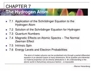
7.1 Application of the Schr ö dinger Equation to the Hydrogen Atom 7.2 Solution of the Schr ö dinger Equation for Hyd

1. CHAPTER 7The Hydrogen Atom • 7.1 Application of the Schrödinger Equation to the Hydrogen Atom • 7.2 Solution of the Schrödinger Equation for Hydrogen • 7.3 Quantum Numbers • 7.4 Magnetic Effects on Atomic Spectra – The Normal Zeeman Effect • 7.5 Intrinsic Spin • 7.6 Energy Levels and Electron Probabilities The atom of modern physics can be symbolized only through a partial differential equation in an abstract space of many dimensions. All its qualities are inferential; no material properties can be directly attributed to it. An understanding of the atomic world in that primary sensuous fashion…is impossible. - Werner Heisenberg

2. 7.1: Application of the Schrödinger Equation to the Hydrogen Atom The approximation of the potential energy of the electron-proton system is electrostatic: Rewrite the three-dimensional time-independent Schrödinger Equation. For Hydrogen-like atoms (He+ or Li++) Replace e2 with Ze2 (Z is the atomic number). Use appropriate reduced mass μ.

3. Application of the Schrödinger Equation Transform to spherical polar coordinates because of the radial symmetry. Insert the Coulomb potential into the transformed Schrödinger equation. Equation 7.3 The potential (central force) V(r) depends on the distance r between the proton and electron.

4. Application of the Schrödinger Equation Equation 7.4 The wave function ψ is a function of r, θ, . Equation is separable. Solution may be a product of three functions. We can separate Equation 7.3 into three separate differential equations, each depending on one coordinate: r, θ, or .

5. 7.2: Solution of the Schrödinger Equation for Hydrogen • Substitute Eq (7.4) into Eq (7.3) and separate the resulting equation into three equations: R(r), f(θ), and g( ). Separation of Variables • The derivatives from Eq (7.4) • Substitute them into Eq (7.3) • Multiply both sides by r2 sin2θ / Rfg Equation 7.7

6. Solution of the Schrödinger Equation -------- azimuthal equation Equation 7.8 Only r and θ appear on the left side and only appears on the right side of Eq (7.7) The left side of the equation cannot change as changes. The right side cannot change with either r or θ. Each side needs to be equal to a constant for the equation to be true. Set the constant −mℓ2 equal to the right side of Eq (7.7) It is convenient to choose a solution to be .

7. Solution of the Schrödinger Equation satisfies Eq (7.8) for any value of mℓ. The solution must be single valued in order to have a valid solution for any , which is mℓto be zero or an integer (positive or negative) for this to be true. If Eq (7.8) were positive, the solution would not be normalized.

8. Solution of the Schrödinger Equation Set the left side of Eq (7.7) equal to −mℓ2 and rearrange it. Everything depends on r on the left side and θ on the right side of the equation.

9. Solution of the Schrödinger Equation ----Radial equation Equation 7.10 ----Angular equation Equation 7.11 Set each side of Eq (7.9) equal to constant ℓ(ℓ + 1). Schrödinger equation has been separated into three ordinary second-order differential equations [Eq (7.8), (7.10), and (7.11)], each containing only one variable.

10. Solution of the Radial Equation • The radial equation is called the associated Laguerre equation and the solutions R that satisfy the appropriate boundary conditions are called associated Laguerre functions. • Assume the ground state has ℓ = 0 and this requires mℓ = 0. Eq (7.10) becomes • The derivative of yields two terms and V is the Coulomb potentials. Write those terms: Equation 7.13

11. Solution of the Radial Equation Equation 7.14 Try a solution A is a normalized constant. a0 is a constant with the dimension of length. Take derivatives of R and insert them into Eq (7.13). To satisfy Eq (7.14) for any r is for each of the two expressions in parentheses to be zero. Set the second parentheses equal to zero and solve for a0. Set the first parentheses equal to zero and solve for E. Both equal to the Bohr result.

12. Quantum Numbers • The appropriate boundary conditions to Eq (7.10) and (7.11) leads to the following restrictions on the quantum numbers ℓ and mℓ: • ℓ = 0, 1, 2, 3, . . . • mℓ = −ℓ, −ℓ + 1, . . . , −2, −1, 0, 1, 2, . ℓ . , ℓ − 1, ℓ • |mℓ| ≤ ℓ and ℓ< 0. • The predicted energy level is n = 1,2,3….. n > l

13. Hydrogen Atom Radial Wave Functions First few radial wave functions Rnℓ Subscripts on R specify the values of n and ℓ.

14. Solution of the Angular and Azimuthal Equations • The solutions for Eq (7.8) are . • Solutions to the angular and azimuthal equations are linked because both have mℓ. • Group these solutions together into functions. ---- spherical harmonics

15. Normalized Spherical Harmonics

16. Solution of the Angular and Azimuthal Equations The radial wave function R and the spherical harmonics Y determine the probability density for the various quantum states. The total wave function depends on n, ℓ, and mℓ. The wave function becomes

17. 7.3: Quantum Numbers The three quantum numbers: • n Principal quantum number • ℓ Orbital angular momentum quantum number • mℓ Magnetic quantum number The boundary conditions: • n = 1, 2, 3, 4, . . . Integer • ℓ = 0, 1, 2, 3, . . . , n − 1 Integer • mℓ = −ℓ, −ℓ + 1, . . . , 0, 1, . . . , ℓ − 1, ℓ Integer The restrictions for quantum numbers: • n > 0 • ℓ < n • |mℓ| ≤ ℓ

18. Principal Quantum Number n • It results from the solution of R(r) in Eq (7.4) because R(r) includes the potential energy V(r). The result for this quantized energy is • The negative means the energy E indicates that the electron and proton are bound together.

19. Radial probability density Radial probability density n2ao

20. z y x Shapes of the spherical harmonics (Images from http://odin.math.nau.edu/~jws/dpgraph/Yellm.html)

21. z y x Shapes of spherical harmonics (2) (Images from http://odin.math.nau.edu/~jws/dpgraph/Yellm.html)

22. Orbital Angular Momentum Quantum Number ℓ • It is associated with the R(r) and f(θ) parts of the wave function. • Classically, the orbital angular momentum with L = mvorbitalr. • ℓ is related to L by . • In an ℓ = 0 state, . It disagrees with Bohr’s semiclassical “planetary” model of electrons orbiting a nucleus L = nħ.

23. Orbital Angular Momentum Quantum Number ℓ • A certain energy level is degenerate with respect to ℓ when the energy is independent of ℓ. • Use letter names for the various ℓ values. • ℓ = 0 1 2 3 4 5 . . . • Letter = s p d f g h . . . • Atomic states are referred to by their n and ℓ. • A state with n = 2 and ℓ = 1 is called a 2p state. • The boundary conditions require n > ℓ.

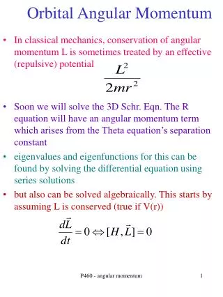
24. Classical angular momentum L p r F For a classical particle, the angular momentum is defined by In components Same origin for r and F Angular momentum is very important in problems involving a central force (one that is always directed towards or away from a central point) because in that case it is conserved

25. Magnetic Quantum Number mℓ • The angle is a measure of the rotation about the z axis. • The solution for specifies that mℓ is an integer and related to the z component of L. • The relationship of L, Lz, ℓ, and mℓ for ℓ = 2. • is fixed because Lz is quantized. • Only certain orientations of are possible and this is called space quantization.

26. z L The vector model This is a useful semi-classical model of the quantum results. Imagine L precesses around the z-axis. Hence the magnitude of L and the z-component Lz are constant while the x and y components can take a range of values and average to zero, just like the quantum eigenfunctions. A given quantum number l determines the magnitude of the vector L via The z-component can have the 2l+1 values corresponding to In the vector model this means that only particular special angles between the angular momentum vector and the z-axis are allowed θ

27. Magnetic Quantum Number mℓ Quantum mechanics allows to be quantized along only one direction in space. Because of the relation L2 = Lx2 + Ly2 + Lz2 the knowledge of a second component would imply a knowledge of the third component because we know . We expect the average of the angular momentum components squared to be .

28. 7.4: Magnetic Effects on Atomic Spectra—The Normal Zeeman Effect • The Dutch physicist Pieter Zeeman showed the spectral lines emitted by atoms in a magnetic field split into multiple energy levels. It is called the Zeeman effect. • A spectral line is split into three lines. • Consider the atom to behave like a small magnet. • Think of an electron as an orbiting circular current loop of I = dq / dt around the nucleus. • The current loop has a magnetic moment μ = IA and the period T = 2πr / v. • where L = mvr is the magnitude of the orbital angular momentum.

29. 7.4: Magnetic Effects on Atomic Spectra—The Normal Zeeman Effect t = m x B = dL/dt

30. The Normal Zeeman Effect • Since there is no magnetic field to align them, point in random directions. The dipole has a potential energy The angular momentum is aligned with the magnetic moment, and the torque between and causes a precession of . Where μB = eħ / 2m is called a Bohr magneton. cannot align exactly in the z direction and has only certain allowed quantized orientations.

31. The Normal Zeeman Effect • The potential energy is quantized due to the magnetic quantum number mℓ. • When a magnetic field is applied, the 2p level of atomic hydrogen is split into three different energy states with energy difference of ΔE = μBB Δmℓ.

32. The Normal Zeeman Effect A transition from 2p to 1s.

33. The Stern-Gerlach Experiment An atomic beam of particles in the ℓ = 1 state pass through a magnetic field along the z direction. The mℓ = +1 state will be deflected down, the mℓ = −1 state up, and the mℓ = 0 state will be undeflected. If the space quantization were due to the magnetic quantum number mℓ, mℓ states is always odd (2ℓ + 1) and should have produced an odd number of lines.

34. 7.5: Intrinsic Spin • Samuel Goudsmit and George Uhlenbeck in Holland proposed that the electron must have an intrinsic angular momentum and therefore a magnetic moment. • Paul Ehrenfest showed that the surface of the spinning electron should be moving faster than the speed of light! • In order to explain experimental data, Goudsmit and Uhlenbeck proposed that the electron must have an intrinsic spin quantum numbers = ½.

35. Intrinsic Spin The electron’s spin will be either “up” or “down” and can never be spinning with its magnetic moment μs exactly along the z axis. The intrinsic spin angular momentum vector . The spinning electron reacts similarly to the orbiting electron in a magnetic field. We should try to find L, Lz, ℓ, and mℓ. The magnetic spin quantum numberms has only two values, ms = ±½.

36. Intrinsic Spin and no splitting due to . there is space quantization due to the intrinsic spin. The magnetic moment is . The coefficient of is −2μB as with is a consequence of theory of relativity. The gyromagnetic ratio (ℓ or s). gℓ = 1 and gs = 2, then The z component of . In ℓ = 0 state Apply mℓ and the potential energy becomes

37. 7.6: Energy Levels and Electron Probabilities • For hydrogen, the energy level depends on the principle quantum number n. • In ground state an atom cannot emit radiation. It can absorb electromagnetic radiation, or gain energy through inelastic bombardment by particles.

38. Selection Rules • We can use the wave functions to calculate transition probabilities for the electron to change from one state to another. Allowed transitions: • Electrons absorbing or emitting photons to change states when Δℓ = ±1. Forbidden transitions: • Other transitions possible but occur with much smaller probabilities when Δℓ ≠ ±1.

39. Probability Distribution Functions • We must use wave functions to calculate the probability distributions of the electrons. • The “position” of the electron is spread over space and is not well defined. • We may use the radial wave function R(r) to calculate radial probability distributions of the electron. • The probability of finding the electron in a differential volume element dτis .

40. Probability Distribution Functions The differential volume element in spherical polar coordinates is Therefore, We are only interested in the radial dependence. The radial probability density is P(r) = r2|R(r)|2 and it depends only on n and l.

41. Probability Distribution Functions • R(r) and P(r) for the lowest-lying states of the hydrogen atom.

42. Probability Distribution Functions The probability density for the hydrogen atom for three different electron states.