LECTURE 15 Hypotheses about Contrasts
LECTURE 15 Hypotheses about Contrasts. EPSY 640 Texas A&M University. Hypotheses about Contrasts. C = c 1 1 + c 2 2 + c 3 3 + …+ c k k , with c i = 0 . The null hypothesis is H 0 : C = 0 H 1 : C 0. Hypotheses about Contrasts.

LECTURE 15 Hypotheses about Contrasts
E N D
Presentation Transcript
LECTURE 15Hypotheses about Contrasts EPSY 640 Texas A&M University
Hypotheses about Contrasts C = c11 + c22 + c33 + …+ ckk , with ci = 0 . The null hypothesis is H0: C = 0 H1: C 0
Hypotheses about Contrasts C1 = (0)instruction + (1)advance organizer (-1)neutral topic Thus, for this contrast we ignore the straight instruction condition, as evidenced by its weight of 0, and subtract the mean of the neutral topic condition from the mean for the advance organizer condition. A second contrast might be 2, -1, -1: C2 = (2)instruction (-1)advance organizer (-1)neutral topic We can interpret this contrast better by examining its null hypothesis: C2 = 0 = (2)instruction (-1)advance organizer (-1)neutral topic , so that (2)instruction = (1)advance organizer + (1)neutral topic and instruction -[ (1)[advance organizer + (1)neutral topic ] / 2 = 0 .
Contrasts • simple contrasts, if only two groups have nonzero coefficients, and • complex contrasts for those involving three or more groups
Planned Orthogonal Contrasts Orthogonal contrasts have the property that they are mathematically independent of each other. That is, there is no information in one that tells us anything about the other. This is created mathematically by requiring that for each pair of contrasts in the set, ci1ci2 = 0, where ci1 is the contrast value for group i in contrast 1, ci2 the contrast value for the same group in contrast 2. For example, with C1 and C2 above, C1 : 0 1 -1 C2: 2 -1 -1 C1C2: 0 x 2 + 1 x –1 + -1 x –1 = 0 –1 + 1 = 0
Planned Orthogonal Contrasts • VENN DIAGRAM REPRESENTATION SSc2 Treat SS SSy R2c1=SSc1/SSy R2c2=SSc2/SSy R2y=(SSc1+SSc2)/SSy SSerror SSc1
Geometry of POCs GP 2 GP 3 C1: 0, 1, -1 C2: 2, -1, -1 GP 1
PATH DIAGRAM FOR PLANNED ORTHOGONAL CONTRASTS C1 1 (rc1,y)=.085 C2 y e 2 (rc2,y) = .048
Nonorthogonal Contrasts • VENN DIAGRAM REPRESENTATION SSc1 Treat SS SSy SSerror SSc2
PATH DIAGRAM FOR PLANNED NONORTHOGONAL CONTRASTS r=.78 C1 1 (rc1,y)=.128 C2 y e 2 (rc2,y) = -.022
Control Treatment Treatment+Drug Treatment+ Placebo C T TD TP The purpose of the placebo is to mimic the results of the drug . An even more complex design might include a control plus the placebo. The set of orthogonal contrasts follow from hypotheses of interest: C T TD TP C1 : 3 -1 -1 -1 This contrast assesses whether treatments are more effective generally than the control condition.
Control Treatment Treatment+Drug Treatment+ Placebo C T TD TP C2: 0 2 -1 -1 This contrast compares the treatment with additions to treatment. C3: 0 0 1 -1 and this contrast compares the effect of the drug with the placebo. There are other sets of contrasts a researcher might substitute or add. Here, we will look at the contrasts to determine that they are orthogonal: C1: 3 -1 -1 -1 C2 0 2 -1 -1 0+ -2 +1 +1 = 0, so that C1 and C2 are orthogonal.
Control Treatment Treatment+Drug Treatment+ Placebo C T TD TP C1: 3 -1 -1 -1 C3 0 0 1 -1 0 + -0 -1+1 = 0, so that C1 and C3 are orthogonal. C3: 0 0 1 -1 C2 0 2 -1 -1 0 + -0 –1 +1 = 0, so that C3 and C2 are orthogonal.
A second set of contrasts might be developed as follows: C T TD TP C1 : 2 -1 -1 0 This contrasts the control with the primary drug conditions of interest. Next, C2: 0 1 -1 0 This contrast compares the treatment with treatment plus drug, the major interest of the study. Finally C3: 0 0 1 -1 and this contrast compares the effect of the drug with the placebo. C1: 2 -1 -1 0 C2 0 1 -1 0 0 +-1 +1+0 = 0, so that C1 and C2 are orthogonal. C1: 2 -1 -1 0 C3 0 0 1 -1 0+ 0 -1+0 = -1, so that C1 and C3 are not orthogonal. C3: 0 0 1 -1 C2 0 1 -1 0 0 + -0 –1 0 = -1, so that C3 and C2 are not orthogonal.
Polynomial Trend Contrasts • When groups represent interval data we can conduct polynomial trend contrasts • example: Group A receives no treatment, Group B 10 hours, and group C receives 20 hours of instructional treatment • Treatment condition (time) is now interval: 0 10 20
Polynomial Trend Contrasts • The contrast coefficients for polynomial trends fit curves: linear, quadratic, cubic, etc. • The coefficients can be obtained from statistics texts most easily • SPSS has a polynomial trend option in the Analyze/Compare Means/One Way ANOVA analysis
Polynomial Trend Contrasts: example of drug dosages 0 100 200 300 ml dose C1 : -3 -1 1 3 linear C2: -1 1 1 -1 quadratic C3: -1 3 -3 1 cubic
C1 3 2 1 0 -1 -2 -3 3 2 1 0 -1 -2 -3 C3 3 2 1 0 -1 -2 -3 C2 0 100 200 300 0 100 200 300 0 100 200 300 Fig. Graphs of planned orthogonal contrasts for four interval treatments
SPSS EXAMPLE The groups represent the five quintiles of school enrollment size, 1-281, 282-443, 444-570, 571-717, and 718-2968
SPSS EXAMPLE Unweighted used because each group has the same # of schools
SPSS EXAMPLE We might have gotten a quadratic from this curve but too much variation within groups