The Dynamics of Learning Vector Quantization

1. The Dynamics of Learning Vector Quantization Barbara Hammer Michael Biehl, Anarta Ghosh TU Clausthal-Zellerfeld Institute of Computing Science Rijksuniversiteit Groningen Mathematics and Computing Science

2. The dynamics of learning a model situation: randomized data learning algorithms for VQ und LVQ analysis and comparison: dynamics, success of learning Summary Outlook Introduction prototype-based learning from example data: representation, classification Vector Quantization (VQ) Learning Vector Quantization (LVQ)

3. example: identification and grouping in clusters of similar data assignment of feature vector  to the closest prototypew (similarity or distance measure, e.g. Euclidean distance ) Vector Quantization (VQ) aim: representation of large amounts of data by (few) prototype vectors

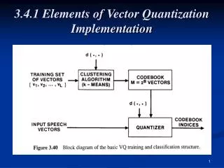
4. • initialize K prototype vectors • present a single example • identify the closest prototype, i.ethe so-calledwinner • move the winner even closertowards the example unsupervised competitive learning intuitively clear, plausible procedure - places prototypes in areas with high density of data - identifies the most relevant combinations of features - (stochastic) on-line gradient descent with respect to the cost function ...

5. quantization error here: Euclidean distance wjis the winner ! prototypes data aim: faithful representation (in general: ≠ clustering ) Result depends on - the number of prototype vectors - the distance measure / metric used

6. , 3 prototypes example situtation: 3 classes assignment of a vector  to the class of the closest prototype w   classification:      aim : generalization ability, i.e. correct classification of novel data after training Learning Vector Quantization (LVQ) aim: classification of data learning from examples Learning: choice of prototypes according to example data

7. • initialize prototype vectors (for different classes) • present a single example • identify the closestcorrect and the closest wrong prototype • move the corresponding winner towards / away from the example mostly: heuristically motivated variations of competitive learning prominent example[Kohonen]: “ LVQ 2.1. ” known convergence / stability problems, e.g. for infrequent classes

8. real time speech recognition • medical diagnosis, e.g. from histological data • gene expression data analysis • texture recognition and classification • . . . LVQ algorithms ... • appear plausible, intuitive, flexible • are fast, easy to implement • are frequently applied in a variety of problems involving • the classification of structured data, a few examples:

9. illustration: microscopic images of (pig) semen cells after freezing and storage, c/o Lidia Sanchez-Gonzalez, Leon/Spain

10. prototypes obtained by LVQ (1) illustration: microscopic images of (pig) semen cells after freezing and storage, c/o Lidia Sanchez-Gonzalez, Leon/Spain damaged cells healthy cells

11. LVQ algorithms ... • are often based on purely heuristic arguments, or derived from a cost function with unclear relation to the generalization ability • almost exclusively use the Euclidean distance measure, • inappropriate for heterogeneous data • lack, in general, a thorough theoretical understanding of • dynamics, convergence properties, • performance w.r.t. generalization, etc.

12. In the following: analysis of LVQ algorithms w.r.t. - dynamics of the learning process - performance, i.e. generalization ability - asymptotic behavior in the limit of many examples typical behavior in a model situation - randomized, high-dimensional data - essential features of LVQ learning aim: - contribute to the theoretical understanding - develop efficient LVQ schemes - test in applications

13. orthonormal center vectors: B+, B-∈ ℝN, ( B )2 =1, B+·B- =0 prior weights of classes p+,p- p+ + p- = 1 (p-) ℓ separation ℓ B- independent components: B+ (p+) model situation: two clusters of N-dimensional data random vectors ∈ ℝN according to mixture of two Gaussians:

14. μ w ξ = × x 2 2 projections in two independent random directions w1,2 (240) (160) μ ξ model for studying typical behavior of LVQ algorithms, not: density-estimation based classification = × y B - - Note: μ w ξ μ × = ξ x = × y B + + 1 1 high-dimensional data (formally: N∞) 400 examples ξμ∈ℝN , N=200, ℓ=1, p+=0.6 projections into the plane of center vectors B+,B- (240) (160)

15. sequence of independent random data acc. to update of prototype vectors: learning rate, step size change of prototype towards or away from the current data competition, direction of update etc. above examples: unsupervised Vector Quantization The Winner Takes It All (classes irrelevant/unknown) Learning Vector Quantization “2.1.” here: two prototypes, no explicit competition dynamics of on-line training

16. 1. description in terms of a few characteristic quantitities ( here: ℝ2N  ℝ7) length and relative position of prototypes projections in the (B+, B-)-plane  recursions projections distances random vector ξμ enters only in the form of mathematical analysis of the learning dynamics

17. correlated Gaussian random quantities random vector acc. to in the thermodynamic limit N    averaged recursionsclosed in { Rsσ, Qst} 2. average over the current example completely specified in terms of first and second moments (w/o indices μ)

18. characteristic quantities - depend on the random sequence of example data - their variance vanishes with N  (here: ∝ N-1) 4. continuous learning time # of examples # of learning steps per degree of freedom recursions  coupled, ordinary differential equations  evolution of projections 3. self-averaging properties learning dynamics is completely described in terms of averages

19. N   investigation and comparison of given algorithms • - repulsive/attractive fixed points of the dynamics • - asymptotic behavior for  • dependence on learning rate, separation, initialization • ... optimization and development of new prescriptions • - time-dependent learning rate η(α) • variational optimization w.r.t. fs[...] • - ... maximize 5. learning curve probability for misclassification of a novel example generalization error εg(α)after training with α N examples

20. in the model situation (equal variances of clusters): separation of classes by the plane with ℓ excess error 0.50 ℓ=0 εg 0.25 ℓ=1 minimal εg as a function of prior weights ℓ=2 0 p+ 1.0 0 0.5 optimal classification with minimal generalization error (p+) B+ B- (p->p+ )

21. p = (1+m  ) / 2 (m>0) (analytical) integration for ws(0) = 0 theory and simulation (N=100) p+=0.8, ℓ=1, =0.5 averages over 100 independent runs “LVQ 2.1.“ update the correct and wrong winner [Seo, Obermeyer]: LVQ2.1. ↔ cost function (likelihood ratios)

22. problem: instability of the algorithm due to repulsion of wrong prototypes trivial classification für α∞: εg = max { p+,p- } strategies: - selection of data in a window close to the current decision boundary slows down the repulsion, system remains instable • Soft Robust Learning Vector Quantization[Seo & Obermayer] • density-estimation based cost function • limiting case Learning from mistakes: LVQ2.1-step only, • if the example is currently misclassified slow learning, poor generalization (p+> p-) (p- )

23. I) LVQ 1 [Kohonen] only the winner is updated according to the class membership 1 winner ws RS+ w- numerical integration for ws(0)=0 ℓ B+ R++ Q++ w+ R-- R-+ Q-- ℓ B- Q+- w- R-- RS- α trajectories in the (B+,B- )-plane (•)=20,40,....140 ....... optimal decision boundary ____ asymptotic position theory and simulation (N=200) p+=0.2, ℓ=1.2, =1.2 averaged over 100 indep. runs “ The winner takes it all ”

24. η 0.26 • role of the learning rate εg εg 0.22 - stationary state: 0.2 0.18 εg (α∞) grows lin. with η η0 0.4 2.0 0.14 200 100 300 0 α  0.26 • well-defined asymptotics: • (ODE linear in η) εg η 0, α∞ ( ηα ) ∞ 0.22 η0 0.18 suboptimal 0.14 min.εg 10 0 30 20 40 50 (ηα) learning curve (p+=0.2, ℓ=1.2) =1.2 - variable rate η(α)!?

25. w+ ℓ B+ classification scheme and the achieved generalization error are independent of the prior weights p (and optimal for p= 1/2 ) ℓ B- w- LVQ+ ≈ VQ within the classes p+=0.2, ℓ=1.2, =1.2 “ The winner takes it all “ II ) LVQ+ ( only positive steps without repulsion) winner correct (wsupdated only from class S) α∞ asymptotic configuration symmetric about ℓ(B++B-)/2

26. εg p+=0.2, ℓ=1.0, =1.0 εg min {p+,p-} • LVQ 1 • here: close to optimal • classification optimal classification α p+ p+ • LVQ+ • min-max solution • p± -independent classification learning curves LVQ+ LVQ1 asymptotics:η0, (ηα)∞ • LVQ 2.1. • trivial assignment to the • more frequent class

27. competitive learning ws winner numerical integration for ws(0)≈0 ( p+=0.2, ℓ=1.0, =1.2 ) R-- system is invariant under exchange of the prototypes  weakly repulsive fixed points εg VQ 1.0 R++ R+- LVQ+ LVQ1 R-+ 0 α α 200 100 α 0 300 Vector Quantization class membership is unknown or identical for all data

28. εg asymptotics (,0, ) p+≈0 p-≈1 p+ - low quantization error - high gen. error εg interpretations: • VQ, unsupervised learning • unlabelled data • LVQ, two prototypes of the • same class, identical labels • LVQ, different classes, but • labels are not used in training

29. Summary • prototype-based learning • Vector Quantization and Learning Vector Quantization • a model scenario: two clusters, two prototypes • dynamics of online training • comparison of algorithms: • LVQ 2.1.: instability, trivial (stationary) classification • LVQ 1 : close to optimal asymptotic generalization • LVQ + : min-max solution w.r.t. asymptotic generalization • VQ : symmetry breaking, representation • work in progress, outlook • regularization of LVQ 2.1, Robust Soft LVQ [Seo, Obermayer] • model: different cluster variances, more clusters/prototypes • optimized procedures: learning rate schedules, • variational approach / density estimation / Bayes optimal on-line • several classes and prototypes

30. Generalized Relevance LVQ [Hammer & Villmann] • adaptive metrics, e.g. distance measure training neighborhood preserving SOM Neural Gas (distance based) Perspectives • Self-Organizing Maps (SOM) • (many) N-dim. prototypes form a (low) d-dimensional grid • representation of data in a topology preserving map • applications