Learning and Vision: Generative Methods
Learning and Vision: Generative Methods. Andrew Blake, Microsoft Research Bill Freeman, MIT ICCV 2003 October 12, 2003 . Learning and vision: Generative Methods. Machine learning is an important direction in computer vision. Our goal for this class: Give overviews of useful techniques.

Learning and Vision: Generative Methods
E N D
Presentation Transcript
Learning and Vision: Generative Methods Andrew Blake, Microsoft Research Bill Freeman, MIT ICCV 2003 October 12, 2003
Learning and vision: Generative Methods • Machine learning is an important direction in computer vision. • Our goal for this class: • Give overviews of useful techniques. • Show how these methods can be used in vision. • Provide references and pointers. • Note afternoon companion class: Learning and vision: Discriminative Methods, taught by Chris Bishop and Paul Viola.
Learning and VisionGenerative Models Intro – roadmap for learning and inference in vision (WTF) Probabilistic inference introduction; integration of sensory data applications: color constancy, Bayes Matte 9:00 Basic estimation methods (WTF) MLE, Expectation Maximization applications: two-line fitting Learning and inference in temporal and spatial Markov processes Techniques: 9.25 (1) PCA, FA, TCA: (AB) inference – linear (Wiener) filter learning: by Expectation Maximization (EM); applications: face simulation, denoising, Weiss’s intrinsic images and furthermore: Active Appearance Models, Simoncelli, ICA & non-Gaussianity, filter banks 10.00 (2) Markov chain & HMM: (AB) inference: - MAP by Dynamic Programming, Forward and Forward-Backward (FB) algorithms; learning: by EM – Baum-Welch; representations: pixels, patches applications: stereo vision and furthermore: gesture models (Bobick-Wilson) < Break 10.30-10.45 > 10.45 (3) AR models: (AB) Inference: Kalman-Filter, Kalman Smoother, Particle Filter; learning: by EM-FB; representations: patches, curves, chamfer maps, filter banks applications: tracking (Isard-Blake, Black-Sidenbladh, Jepson-Fleet-El Maraghi); Fitzgibbon-Soatto textures and furthermore: EP 11.30 (4) MRFs: (WTF) Inference: ICM, LoopyBelief Propagation (BP), Generalised BP,Graph Cuts; Parameter learning: Pseudolikelihood maximisation; representations:color pixels, patches applications: Texture segmentation, super resolution (Freeman-Pasztor), distinguishing shading from paint and furthermore: Gibbs sampling, Discriminative Random Field (DRF), low level segmentation (Zhu et al.)
What is the goal of vision? If you are asking, “Are there any faces in this image?”, then you would probably want to use discriminative methods.
What is the goal of vision? If you are asking, “Are there any faces in this image?”, then you would probably want to use discriminative methods. If you are asking, “Find a 3-d model that describes the runner”, then you would use generative methods.
Modeling So we want to look at high-dimensional visual data, and fit models to it; forming summaries of it that let us understand what we see.
Posterior probability Likelihood function Prior probability mean data points std. dev. Evidence By Bayes rule How find the parameters of the best-fitting Gaussian?
Posterior probability Likelihood function Prior probability mean data points std. dev. Evidence Maximum likelihood parameter estimation: How find the parameters of the best-fitting Gaussian?
Derivation of MLE for Gaussians Observation density Log likelihood Maximisation
Basic Maximum Likelihood Estimate (MLE) of a Gaussian distribution Mean Variance Covariance Matrix
Basic Maximum Likelihood Estimate (MLE) of a Gaussian distribution Mean Variance For vector-valued data, we have the Covariance Matrix
Maximum likelihood estimation for the slope of a single line Data likelihood for point n: Maximum likelihood estimate: where gives regression formula
Model fitting example 3:Fitting two lines to observed data y x
MLE for fitting a line pair (a form of mixture dist. for )
Line 1 Line 2 Fitting two lines: on the one hand… If we knew which points went with which lines, we’d be back at the single line-fitting problem, twice. y x
Fitting two lines, on the other hand… We could figure out the probability that any point came from either line if we just knew the two equations for the two lines. y x
Expectation Maximization (EM): a solution to chicken-and-egg problems
MLE with hidden/latent variables:Expectation Maximisation General problem: data parameters hidden variables For MLE, want to maximise the log likelihood The sum over z inside the log gives a complicated expression for the ML solution.
The EM algorithm We don’t know the values of the labels, zi , but let’s use its expected value under its posterior with the current parameter values, old. That gives us the “expectation step”: “E-step” Now let’s maximize this Q function, an expected log-likelihood, over the parameter values, giving the “maximization step”: “M-step” Each iteration increases the total log-likelihood log p(y|)
Expectation Maximisation applied to fitting the two lines Need: /2 and then: and maximising that gives associate data point with line Hidden variables and probabilities of association are : ’ ’
EM fitting to two lines with /2 “E-step” and repeat Regression becomes: “M-step”
Experiments: EM fitting to two lines (from a tutorial by Yair Weiss, http://www.cs.huji.ac.il/~yweiss/tutorials.html) Line weights line 1 line 2 Iteration 1 2 3
Applications of EM in computer vision • Structure-from-motion with multiple moving objects • Motion estimation combined with perceptual grouping • Multiple layers/or sprites in an image.