Exploring Descriptive Statistics: Data Presentation and Inference
Discover the essence of statistical inference from data and learn the art of presenting data effectively through various techniques like bar charts, histograms, and boxplots. Dive into examples relating to machine breakdowns and defective computer chips to understand the significance of sample representation and population selection. Explore sample statistics such as mean, median, variance, and quantiles to glean insights from datasets. Unveil the intriguing relationship between the sample mean, median, and trimmed mean for skewed data sets. Enhance your understanding of data analysis and statistical interpretation in this comprehensive guide to descriptive statistics.

Exploring Descriptive Statistics: Data Presentation and Inference
E N D
Presentation Transcript
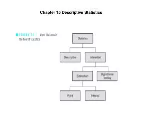
Chapter 6. Descriptive Statistics 6.1 Experimentation 6.2 Data Presentation 6.3 Sample Statistics 6.4 Examples
Data: a mixture of nature and noise. • Is the noise manageable? • The noise is desired to be represented by a probability distribution. • Statistical inference: • The science of deducing properties of an underlying probability distribution from data • Can we have information on the underlying probability distribution? • The information is given in the form of (functions of) data.
Figure 6.1 The relationship between probability theory and statistical inference
6.1 Experimentation6.1.1 Samples • Population: the set of all the possible observations available from a particular probability distribution. • Sample: a subset of a population. • Random sample: a sample where the elements are chosen at random from the population • A sample is desired to be representative of the population. • Types of observations: numerical and nominal x
6.1.2 Examples • Example 1: Machine breakdowns • Suppose that an engineer in charge of the maintenance of a machine keeps records on the breakdown causes over a period of a year. • Suppose that 46 breakdowns were observed by the engineer (see Figure 6.2). • What is the population from which this sample is drawn? • Factors to consider to check the representative of data: • Quality of operators • Working load on the machine • Particularity of data observation (e.g., more rainy days than other years)
Example 2: Defective computer chips • The chip boxes are selected at random from ….. • Points to check on data: • What is the data type? • Are the data representative? • How the randomness of data realized? • Statistical problem: • What is the population from which the data are sampled?
6.2 Data presentation 6.2.1 Bar and Pareto charts 6.2.2 Pie charts 6.2.3 Histograms 6.2.4 Outliers • An outlier is an observation which is not from the distribution from which the main body of the sample is collected.
Figure 6.9 Pareto chart of customer complaints for Internet company
Figure 6.16 Histograms of metal cylinder diameter data set with different bandwidths
6.3 Sample statistics 6.3.1 Sample mean 6.3.2 Sample median 6.3.3 Sample trimmed mean 6.3.4 Sample mode 6.3.5 Sample variance 6.3.6 pth Sample quantiles 6.3.7 Boxplots
Cf. Chebyshev’s inequality: Let Then, In general, Cf. Theorem: the weak law of large numbers Let be a sequence of i.i.d. random variables, each having mean and variance Then, for any
Figure 6.23Relationship between the samplemean, median, and trimmed meanfor positively and negativelyskeweddata sets
Figure 6.33 Boxplot and summary statistics for rolling mill scrap data set