Download
1 / 58
580 likes | 706 Vues
Review last lectures. centrifugal (fly-ball) governor. 1788 Picture shows an operation principle of the fly-ball (centrifugal) speed governor developed by James Watt. simple feedback system. heat transfer Q out. desired temperature. _. room temperature. Q in. S. thermostat. switch.

E N D
centrifugal (fly-ball) governor 1788Picture shows an operation principle of the fly-ball (centrifugal) speed governor developed by James Watt.
simple feedback system heat transfer Qout desired temperature _ room temperature Qin S thermostat switch air con office room +
closed-loop (feedback) system error oractuating signal input orreference disturbance summing junctionor comparator plant output orcontrolledvariable controlsignal + S input filter(transducer) controller actuator process _ sensor oroutput transducer sensor noise
open-loop system input orreference disturbance plant output orcontrolledvariable controlsignal input filter(transducer) controller actuator process
Example 1: Liquid Level System (input flow) Goal: Design the input valve control to maintain a constant height regardless of the setting of the output valve Input valve control float (resistance) (height) (output flow) Output valve (volume)
Users RPCs Tuning Reference control value Sensor Controller Server Log Administrator Server Queue Length Example 2: Admission Control Goal: Design the controller to maintain a constant queue length regardless of the workload
Why Control Theory • Systematic approach to analysis and design • Transient response • Consider sampling times, control frequency • Taxonomy of basic controls • Select controller based on desired characteristics • Predict system response to some input • Speed of response (e.g., adjust to workload changes) • Oscillations (variability) • Approaches to assessing stability and limit cycles
Controller Design Methodology Start System Modeling Controller Design Block diagram construction Controller Evaluation Transfer function formulation and validation Objective achieved? Stop Y Model Ok? N Y N
Control System Goals • Regulation • thermostat, target service levels • Tracking • robot movement, adjust TCP window to network bandwidth • Optimization • best mix of chemicals, minimize response times
Approaches to System Modelling • First Principles • Based on known laws • Physics, Queuing theory • Difficult to do for complex systems • Experimental (System ID) • Statistical/data-driven models • Requires data • Is there a good “training set”?
Laplace transforms • The Laplace transform of a signal f(t) is defined as • The Laplace transform is an integral transform that changes a function of tto a function of a complex variable s = s+ jw • The inverse Laplace transform changes the function of sback to a function of t
Laplace transforms of basic functions f(t) = 0, t < 0 Note:
Example f (t) Laplace transform: signal 1 t 0 w w s s
Properties of Laplace transforms • Linear operator: if and then for any two signals f1(t)and f2(t) and any two constants a1and a2 • Time delay:
Properties of Laplace transforms cont. • Laplace transforms of derivatives: if then
Properties of Laplace transforms cont. • Laplace transform of integrals: • The Laplace transform changes differential equations in t into arithmetic equations in s
Using Laplace transforms to solve ODEs • The Laplace transform can be used to solve differential equations • Method: • Transform the differential equation into the ‘Laplace domain’ (equation in t→ equation ins) • Rearrange to get the solution • Transform the solution back from the Laplace domain to the time domain (signal in s→ signal int) • Usually the Laplace transform (step 1) and the inverse transform (step 3) are done using a Table of Laplace transforms
Example • Use Laplace transforms to find the unforced response of a spring-mass-damper with initial conditions x m = 1 kg k = 2 N/m b = 3 Ns/m k m f b x Equation of motion m f Free body diagram
Example – solution • Take Laplace transform of both sides of equation of motion: • Equation of motion in Laplace domain is
Rearrange: • Apply initial conditions: External force Initial conditions • The system can be in motion if • An external force is applied • The initial conditions are not an equilibrium state (not zero)
Partial fraction expansion: • Use tables to find inverse Laplace transform • System response (in time domain) is x(t) x0 t 0
Partial fraction expansion • A partial fraction expansion can be used to find the inverse transform of • This can be expanded as • Note that • So
Example - Partial fraction expansion • Find the partial fraction expansion of • This can be expanded as • So
Other examples 1. 2. 3.
Insights from Laplace Transforms • What the Laplace Transform says about f(t) • Value of f(0) • Initial value theorem • Does f(t) converge to a finite value? • Poles of F(s) • Does f(t) oscillate? • Poles of F(s) • Value of f(t) at steady state (if it converges) • Limiting value of F(s) as s ---> 0
Transfer Function • Definition • H(s) = Y(s) / X(s) • Relates the output of a linear system (or component) to its input • Describes how a linear system responds to an impulse • All linear operations allowed • Scaling, addition, multiplication H(s) X(s) Y(s)
Block Diagrams • Pictorially expresses flows and relationships between elements in system • Blocks may recursively be systems • Rules • Cascaded (non-loading) elements: convolution • Summation and difference elements • Can simplify
Block Diagram of System Disturbance Reference Value + S S Plant Controller – Transducer
Combining Blocks Reference Value + S Combined Block – Transducer
Key Transfer Functions Reference + Plant Controller S – Transducer