UNIT – 1 Data Preprocessing
UNIT – 1 Data Preprocessing. Data Preprocessing. Learning Objectives Understand why preprocess the data. Understand how to clean the data. Understand how to integrate and transform the data. Why preprocess the data? Data cleaning Data integration and transformation.

UNIT – 1 Data Preprocessing
E N D
Presentation Transcript
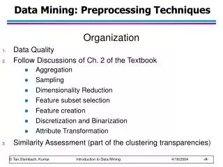
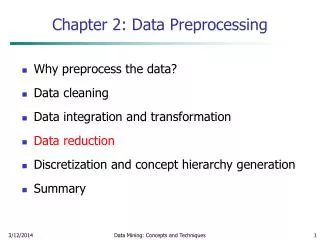
Data Preprocessing Learning Objectives • Understand why preprocess the data. • Understand how to clean the data. • Understand how to integrate and transform the data. • Why preprocess the data? • Data cleaning • Data integration and transformation
Why Data Preprocessing? • Data mining aims at discovering relationships and other forms of knowledge from data in the real world. • Data map entities in the application domain to symbolic representation through a measurement function • Data in the real world is dirty incomplete: missing data, lacking attribute values, lacking certain attributes of interest, or containing only aggregate data noisy: containing errors, such as measurement errors, or outliers inconsistent: containing discrepancies in codes or names distorted: sampling distortion (A Change for worse) 4. No quality data, no quality mining results! (GIGO) 5. Quality decisions must be based on quality data 6. Data warehouse needs consistent integration of quality data
Multi-Dimensional Measure of Data Quality • Data quality is multidimensional: • Accuracy • Preciseness (=reliability) • Completeness • Consistency • Timeliness • Believability (=validity) • Value added • Interpretability • Accessibility • Broad categories: • intrinsic, contextual, representational, and accessibility
Major Tasks in Data Preprocessing • Data cleaning • Fill in missing values, smooth noisy data, identify or remove outliers, and resolve inconsistencies and errors • Data integration • Integration of multiple databases, data cubes, or files • Data transformation • Normalization and aggregation • Data reduction • Obtains reduced representation in volume but produces the same or similar analytical results • Data discretization • Part of data reduction but with particular importance, especially for numerical data
2. Descriptive Data Summarization • For data preprocessing to be successful, it is essential to have an overall picture of your data. • Descriptive data summarization techniques can be used to identify the typical properties of your data and highlight which data values should be treated as noise or outliers. • Thus, we first introduce the basic concepts of descriptive data summarization before getting into the concrete workings of data preprocessing techniques. • For many data preprocessing tasks, users would like to learn about data characteristics regarding both central tendency and dispersion of the data.
Measures of central tendency include mean, median, mode, and midrange, while measures of data dispersion include quartiles, interquartile range (IQR), and variance. • These descriptive statistics are of great help in understanding the distribution of the data. • Such measures have been studied extensively in the statistical literature. • From the data mining point of view, we need to examine how they can be computed efficiently in large databases. • In particular, it is necessary to introduce the notions of distributive measure, algebraic measure, and holistic measure. • Knowing what kind of measure we are dealing with can help us choose an efficient implementation for it.
2.1 Measuring the Central Tendency In this section, we look at various ways to measure the central tendency of data. The most common and most effective numerical measure of the “center” of a set of data is the (arithmetic) mean. meanmode = 3(meanmedian).
2.2 Measuring the Dispersion of Data • The degree to which numerical data tend to spread is called the dispersion, or variance of the data. The most common measures of data dispersion are • 1) Range, Quartiles, Outliers, and Boxplots • 2) Variance and Standard Deviation • The range of the set is the difference between the largest (max()) and smallest (min()) values. • The most commonly used percentiles other than the median are quartiles. The first quartile, denoted by Q1, is the 25th percentile; the third quartile, denoted by Q3, is the 75th percentile. The quartiles, including the median, give some indication of the center, spread, and shape of a distribution. The distance between the first and third quartiles is a simple measure of spread that gives the range covered by the middle half of the data.
Boxplots are a popular way of visualizing a distribution. A boxplot incorporates the five-number summary as follows: • Typically, the ends of the box are at the quartiles, so that the box length is the interquartile range, IQR. • The median is marked by a line within the box. • Two lines (called whiskers) outside the box extend to the smallest (Minimum) and largest (Maximum) observations.
2.3 Graphic Displays of Basic Descriptive Data Summaries Aside from the bar charts, pie charts, and line graphs used in most statistical or graphical data presentation software packages, there are other popular types of graphs for the display of data summaries and distributions. These include histograms, quantile plots, q-q plots, scatter plots, and loess curves. Such graphs are very helpful for the visual inspection of your data.
3. Data Cleaning • Data cleaning tasks Fill in missing values Identify outliers and smooth out noisy data Correct inconsistent data • Missing Data • Data is not always available a. E.g., many tuples have no recorded value for several attributes, such as customer income in sales data • Missing data may be due to a. equipment malfunction b. inconsistent with other recorded data and thus deleted c. data not entered due to misunderstanding d. certain data may not be considered important at the time of entry e. not register history or changes of the data f. Missing data may need to be inferred.
How to Handle Missing Data? • Ignore the tuple: usually done when class label is missing (assuming the tasks in classification—not effective when the percentage of missing values per attribute varies considerably.) • Fill in the missing value manually: tedious + infeasible? • Use a global constant to fill in the missing value: e.g., “unknown”, a new class?! • Use the attribute mean to fill in the missing value • Use the attribute mean for all samples belonging to the same class to fill in the missing value: smarter • Use the most probable value to fill in the missing value: inference-based such as Bayesian formula or decision tree
2. Noisy Data • Noise: random error or variance in a measured variable • Incorrect attribute values may be due to • faulty data collection instruments • data entry problems • data transmission problems • technology limitation • inconsistency in naming convention • Other data problems which requires data cleaning • duplicate records • inconsistent data
How to Handle Noisy Data? • Binning method: - first sort data and partition into (equi-depth) bins - then one can smooth by bin means, smooth by bin median, - smooth by bin boundaries, etc. • Clustering - detect and remove outliers • Combined computer and human inspection - detect suspicious values and check by human • Regression - smooth by fitting the data into regression functions
Binning Methods for Data Smoothing Sorted data for price (in dollars): 4,8,9,15, 21, 21, 24, 25, 26, 28, 29, 34 * Partition into (equi-depth) bins: - Bin 1: 4, 8, 9, 15 - Bin 2: 21, 21, 24, 25 - Bin 3: 26, 28, 29, 34 * Smoothing by bin means: - Bin 1: 9, 9, 9, 9 - Bin 2: 23, 23, 23, 23 - Bin 3: 29, 29, 29, 29 * Smoothing by bin boundaries: - Bin 1: 4, 4, 4, 15 - Bin 2: 21, 21, 25, 25 - Bin 3: 26, 26, 26, 34
Data Integration • Data integration: • combines data from multiple sources into a coherent store • Schema integration • integrate metadata from different sources • entity identification problem: identify real world entities from multiple data sources, e.g., A.cust-id B.cust-# • Detecting and resolving data value conflicts • for the same real world entity, attribute values from different sources are different • possible reasons: different representations, different scales, e.g., metric vs. British units
Handling Redundant Data in Data Integration • Redundant data occur often when integration of multiple databases • The same attribute may have different names in different databases • One attribute may be a “derived” attribute in another table, e.g., annual revenue • Redundant data may be able to be detected by correlational analysis • Careful integration of the data from multiple sources may help reduce/avoid redundancies and inconsistencies and improve mining speed and quality
Data Transformation • Smoothing: remove noise from data • Aggregation: summarization, data cube construction • Generalization: concept hierarchy climbing • Normalization: scaled to fall within a small, specified range • min-max normalization • z-score normalization • normalization by decimal scaling • Attribute/feature construction • New attributes constructed from the given ones
Data Transformation: Normalization • min-max normalization • z-score normalization • normalization by decimal scaling Where j is the smallest integer such that Max(| |)<1
Data Transformation: Normalization • Min-max normalization: to [new_minA, new_maxA] • Ex. Let income range $12,000 to $98,000 normalized to [0.0, 1.0]. Then $73,600 is mapped to • Z-score normalization (μ: mean, σ: standard deviation): • Ex. Let μ = 54,000, σ = 16,000. Then • Normalization by decimal scaling Where j is the smallest integer such that Max(|ν’|) < 1
5. Data Reduction • Data reduction techniques can be applied to obtain a reduced representation of the data set that is much smaller in volume, yet closely maintains the integrity of the original data. That is, mining on the reduced data set should be more efficient yet produce the same (or almost the same) analytical results.
Strategies for data reduction include the following: • Data cube aggregation, where aggregation operations are applied to the data in the construction of a data cube. 2. Attribute subset selection, where irrelevant, weakly relevant, or redundant attributes or dimensions may be detected and removed. 3. Dimensionality reduction, where encoding mechanisms are used to reduce the data set size. 4. Numerosity reduction, where the data are replaced or estimated by alternative, smaller data representations such as parametric models (which need store only the model parameters instead of the actual data) or nonparametric methods such as clustering, sampling, and the use of histograms. 5. Discretization and concept hierarchy generation, where rawdata values for attributes are replaced by ranges or higher conceptual levels.
5.2 Attribute Subset Selection • Attribute subset selection reduces the data set size by removing irrelevant or redundant attributes (or dimensions). • The goal of attribute subset selection is to find a minimum set of attributes such that the resulting probability distribution of the data classes is as close as possible to the original distribution obtained using all attributes. • Mining on a reduced set of attributes has an additional benefit. • It reduces the number of attributes appearing in the discovered patterns, helping to make the patterns easier to understand.
The “Best” (and “Worst”) attributes are typically determined using tests of statistical significance, which assume that the attributes are independent of one. Many other attribute evaluation measures can be used, such as the information gain measure used in building decision trees for classification
Basic heuristic methods of attribute subset selection include the following techniques, some of which are illustrated in Figure. • 1. Stepwise forward selection: The procedure starts with an empty set of attributes as the reduced set. The best of the original attributes is determined and added to the reduced set. At each subsequent iteration or step, the best of the remaining original attributes is added to the set. • 2. Stepwise backward elimination: The procedure starts with the full set of attributes. At each step, it removes the worst attribute remaining in the set. • 3. Combination of forward selection and backward elimination: The stepwise forward selection and backward elimination methods can be combined so that, at each step, the procedure selects the best attribute and removes the worst from among the remaining attributes.
4. Decision tree induction: Decision tree algorithms, such as ID3, C4.5, and CART, were originally intended for classification. Decision tree induction constructs a flow chart like structure where each internal (non leaf) node denotes a test on an attribute, each branch corresponds to an outcome of the test, and each external (leaf) node denotes a class prediction. At each node, the algorithm chooses the “best” attribute to partition the data into individual classes. When decision tree induction is used for attribute subset selection, a tree is constructed from the given data. All attributes that do not appear in the tree are assumed to be irrelevant. The set of attributes appearing in the tree form the reduced subset of attributes. • The stopping criteria for the methods may vary. The procedure may employ a threshold on the measure used to determine when to stop the attribute selection process.
5.3 Dimensionality Reduction • In dimensionality reduction, data encoding or transformations are applied so as to obtain a reduced or “compressed” representation of the original data. If the original data can be reconstructed from the compressed data without any loss of information, the data reduction is called lossless. If, instead, we can reconstruct only an approximation of the original data, then the data reduction is called lossy. There are several well-tuned algorithms for string compression. Although they are typically lossless, they allow only limited manipulation of the data. • In this section, we instead focus on two popular and effective methods of lossy dimensionality reduction: wavelet transforms and principal components analysis.
Wavelet transforms can be applied to multidimensional data, such as a data cube. • This is done by first applying the transform to the first dimension, then to the second, and so on. The computational complexity involved is linear with respect to the number of cells in the cube. Wavelet transforms give good results on sparse or skewed data and on data with ordered attributes. Lossy compression by wavelets is reportedly better than JPEG compression, the current commercial standard. Wavelet transforms have many real-world applications, including the compression of fingerprint images, computer vision, analysis of time-series data, and data cleaning.
PCA is computationally inexpensive, can be applied to ordered and unordered attributes, and can handle sparse data and skewed data. Multidimensional data of more than two dimensions can be handled by reducing the problem to two dimensions. Principal components may be used as inputs to multiple regression and cluster analysis. • In comparison with wavelet transforms, PCA tends to be better at handling sparse data, whereas wavelet transforms are more suitable for data of high dimensionality.
4 Numerosity Reduction • “Can we reduce the data volume by choosing alternative, ‘smaller’ forms of data representation?” • Techniques of numerosity reduction can indeed be applied for this purpose. These techniques may be parametric or nonparametric. • For parametric methods, a model is used to estimate the data, so that typically only the data parameters need to be stored, instead of the actual data. (Outliers may also be stored.) Log-linear models, which estimate discrete multidimensional probability distributions, are an example. • Nonparametric methodsfor storing reduced representations of the data include histograms, clustering, and sampling. • Let’s look at each of the numerosity reduction techniques mentioned above.
Data Reduction Method (1): Regression and Log-Linear Models • Linear regression: Data are modeled to fit a straight line • Often uses the least-square method to fit the line • Multiple regression: allows a response variable Y to be modeled as a linear function of multidimensional feature vector • Log-linear model: approximates discrete multidimensional probability distributions
Regress Analysis and Log-Linear Models • Linear regression: Y = w X + b • Two regression coefficients, w and b, specify the line and are to be estimated by using the data at hand • Using the least squares criterion to the known values of Y1, Y2, …, X1, X2, …. • Multiple regression: Y = b0 + b1 X1 + b2 X2. • Many nonlinear functions can be transformed into the above • Log-linear models: • The multi-way table of joint probabilities is approximated by a product of lower-order tables • Probability: p(a, b, c, d) = ab acad bcd
Histograms : Histograms use binning to approximate data distributions and are a popular form of data reduction. A histogram for an attribute, A, partitions the data distribution of A into disjoint subsets, or buckets. If each bucket represents only a single attribute-value/frequency pair, the buckets are called singleton buckets. Often, buckets instead represent continuous ranges for the given attribute.
There are several partitioning rules, including the following: Equal-width: In an equal-width histogram, the width of each bucket range is uniform Equal-frequency (or equidepth): In an equal-frequency histogram, the buckets are created so that, roughly, the frequency of each bucket is constant (that is, each bucket contains roughly the same number of contiguous data samples). V-Optimal: If we consider all of the possible histograms for a given number of buckets, the V-Optimal histogram is the one with the least variance. Histogram variance is a weighted sum of the original values that each bucket represents, where bucket weight is equal to the number of values in the bucket. MaxDiff: In a MaxDiff histogram, we consider the difference between each pair of adjacent values.
Clustering Clustering techniques consider data tuples as objects. They partition the objects into groups or clusters, so that objects within a cluster are “similar” to one another and “dissimilar” to objects in other clusters. In data reduction, the cluster representations of the data are used to replace the actual data. The effectiveness of this technique depends on the nature of the data. It is much more effective for data that can be organized into distinct clusters than for smeared data.
Data Reduction Method (3): Clustering • Partition data set into clusters based on similarity, and store cluster representation (e.g., centroid and diameter) only • Can be very effective if data is clustered but not if data is “smeared” • Can have hierarchical clustering and be stored in multi-dimensional index tree structures • There are many choices of clustering definitions and clustering algorithms • Cluster analysis will be studied in depth later
Sampling Sampling can be used as a data reduction technique because it allows a large data set to be represented by a much smaller random sample (or subset) of the data. Suppose that a large data set, D, contains N tuples. Let’s look at the most common ways that we could sample D for data reduction. An advantage of sampling for data reduction is that the cost of obtaining a sample is proportional to the size of the sample sampling complexity is potentially sublinear to the size of the data.
For a fixed sample size, sampling complexity increases only linearly as the number of data dimensions. • When applied to data reduction, sampling is most commonly used to estimate the answer to an aggregate query.
Data Reduction Method (4): Sampling • Sampling: obtaining a small sample s to represent the whole data set N • Allow a mining algorithm to run in complexity that is potentially sub-linear to the size of the data • Choose a representative subset of the data • Simple random sampling may have very poor performance in the presence of skew • Develop adaptive sampling methods • Stratified sampling: • Approximate the percentage of each class (or subpopulation of interest) in the overall database • Used in conjunction with skewed data • Note: Sampling may not reduce database I/Os (page at a time)

