Download
1 / 132
1.33k likes | 1.52k Vues
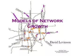
Models of Network Growth. David Levinson. Research Assistants Wei Chen Wenling Chen Ramachandra Karamalaputi Norah Montes de Oca Pavithra Parthasarathi Feng Xie Bhanu Yerra (Dr.) Lei Zhang Shanjiang Zhu. Funding Sources

E N D
Models of Network Growth David Levinson
Research Assistants Wei Chen Wenling Chen Ramachandra Karamalaputi Norah Montes de Oca Pavithra Parthasarathi Feng Xie Bhanu Yerra (Dr.) Lei Zhang Shanjiang Zhu Funding Sources Minnesota Department of Transportation “If They Come, Will You Build It?” Minnesota Department of Transportation “Beyond Business as Usual: Ensuring the Network We Want Is The Network We Get” University of Minnesota Department of Civil Engineering Sommerfeld Fellowship Program Hubert Humphrey Institute of Public Affairs Sustainable Transportation Applied Research Initiative/ University of Minnesota ITS Institute/ U.S. DOT NSF CAREER Award Digital Media Center: Technology Enhanced Learning Grant Acknowledgements
Questions • Why do networks expand and contract? • Do networks self-organize into hierarchies? • Are roads an emergent property? • Can investment rules predict location of network expansions and contractions? • How can this improved knowledge help in planning transportation networks?
Objectives • Model the rise and fall of transportation networks • Study the interdependence of road supply and travel demand at the microscopic level • Demonstrate the model on the Twin Cities transportation network • Apply the model to evaluate alternative transportation investment and pricing policies • Use the model in the classroom
If They Come, Will You Build It? If They Come, Will You Build It?
Agent-Based Modeling • “An agent is an encapsulated computer system that is situated in some environment and that is capable of flexible, autonomous action in that environment in order to meet its design objectives” - Nikolic • Agents can be: Links, Nodes, Travelers, Land • Agent properties • Rules of interaction that determine the state of agents in the next time step • Spatial pattern of interaction between agents • External forces and variables • Initial states
Layered Models • System is split into two layers • Network layer • Land use layer • Network is modeled as a directed graph • Land use layer has small land blocks as agents that represent the population and land use
Flowchart of the simulation model Scope • Exogenous: • economic growth • land use dynamics • Endogenous: • travel behavior/ demand • link maintenance and expansion costs • network revenue (pricing) • investment • induced supply • induced demand
Network • Grid network • Finite Planar Grid • Cylindrical network • Torus network • Modified (Interrupted) Grid • Realistic Networks (Twin Cities) • Initial speed distribution • Every link with same initial speed • Uniformly distributed speeds • Actual network speeds Ideal Chinese Plan
Land Use & Demography • Small land blocks • Population, business activity, and geographical features are attributes • Uniformly and bell-shaped distributed land use are modeled • Actual Twin Cities land use is also tested • Land use is assumed exogenous (future research aimed at testing endogenous land use)
Trip Generation • Using land use model trips produced and attracted are calculated for each cell • Cells are assigned to network nodes using voronoi diagram • Trips produced and attracted are calculated for a network node using voronoi diagram
Calculates trips between network nodes Gravity model Working on agent-based trip distribution Where: Trs is trips from origin node r to destination node s, pris trips produced from node r, qsis trips attracted to node s, drsis cost of travel between nodes r and s along shortest path w is “friction factor” Trip Distribution
Wardrop’s User Equilibrium Principle, travelers choose path with least generalized cost of traveling (s.t. all other travelers also choosing the least cost path) Cases No Congestion Dijkstras Algorithm With Congestion Origin Based Assignment (Boyce & Bar-Gera) Stochastic User Equilibrium (Dial) Agent-based Assignment (Zhang and Levinson, Zhu and Levinson) Flow on a link is Where a,rs = 1 if a Krs, 0 otherwise Krsis a set of links along the shortest path from node r to node s, Route Choice
Generalized link travel cost function la is length of link va is speed of link a l is value of time ta is “toll” q1, q2 are coefficients In No Congestion Case, q1 =0 Link-Performance Function VOT•BPR travel time + Toll
Toll is the only source of revenue Annual revenue generated by a link is total toll paid by the travelers Initially assume only one type of cost, function of length, flow, link speed Revenue And Cost Models
A link based model Speed of a link improves if revenue is more than cost of maintenance, drops otherwise Where: vat is speed of link a at time step t, b is speed reduction coefficient. No revenue sharing between links: Revenue from a link is used in its own investment Network Investment Model (1)
Initial Assumptions • Base case • Network - speed ~ U(1, 1) • Land use ~ U(10, 10) • Friction factor w=0.01 • Travel cost, Revenue da {l= 1.0, o = 1.0, 1 = 1.0, 2 = 0.0} • Infrastructure Cost {m =365, 1 = 1.0, 2 = 0.75, 3 = 0.75} • Investment model { = 1.0} • Speeds on links running in opposite direction between same nodes are averaged
Case 1: Base 15x15 Initial network Equilibrium network state after 9 iterations Slow Fast Figure 5 Equilibrium speed distribution for the base case on a 15x15 grid network
Initial network Equilibrium network state after 8 iterations Slow Fast Figure 7 Equilibrium speed distribution for case 2 on a 15x15 grid network Case 2: Same as base case but initial speeds ~ U(1, 5)
Initial network Equilibrium network state after 7 iterations Slow Fast Figure 9 Equilibrium speed distribution for case 3 on a 15x15 grid network Case 3: Base case with a downtown
Case 7: Self-Fulfilling Investments • Invest in what is normally (base case) lowest volume links. • Results in that being highest volume link. • Decisions do matter: Can use investment to direct outcome.
Four Twin Cities Experiments • Value of time = $10/hr - MnDOT Value • Link performance function 1 = 0.15; 2 =4 - BPR Function • Friction factor =0.1 - Empirical • Revenue Model {1 = 1.0, 2 = 1.0, 3 = 0.75} • Infrastructure Cost { =365, 1 =20, 2 = 1, 3 = 1.25} -CRS in link length, DRS in speed • Coefficient in speed-capacity regression model (1 = -30.6, 2=9.8) - Empirical • Improvement model { = 0.75} DRS in link expansion • CRS, DRS, IRS = Constant, Decreasing, Increasing Returns to Scale
Results Experiment 2: predicted 1998 network Experiment 1: predicted 1998 network Experiment 3: predicted 1998 network Experiment 4: predicted 1998 network
Forecasting Investment Decisions • Build empirically-based network growth prediction models that address the questions: • Will “business as usual” network construction decision rules produce desirable networks? • Will new decision rules produce improved networks? • Should policies be changed to direct future network growth in a better direction? • Should policies be changed to produce networks that will generate the best performance measures? • Results would let decision makers see how current investment decision rules impact or limit future choices.
Processes * Structured process * Ranking system through point allocation * Task forces-committees • Formal • * Priorities • safety,preservation, capacity, • social and economic impacts, • community and agency involvement • Benefit/cost ratio, etc. • * No Ranking System • Informal
Informal Processes • Jurisdictions priorities and decision making: • “ benefit/cost ratio > 1” • “ AADT > 15,000 on 3-lane roadways” (safety reasons) • “ Intersection volumes exceed 7,500 vehicles per day” • “Implementation of policy, strategy and investment level” • “Project development time” • “Most beneficial project for the system” • “Matching funds from local jurisdictions”
Flowcharts-Informal processes Roadways under County’s jurisdiction Scott County Project solicitation Application review Average Daily Traffic (ADT) Safety yes ADT>15,000 3 lane-roads Project in top 200 high crash location list no yes yes no Reapplication? Project approval no no End yes Project construction
Flowcharts - Formal Processes - City Minneapolis streets Project solicitation Application review Compute scores Highest scored project selection yes Allocation of funding availability Reapplication? Project approval no no End yes City of Minneapolis Project construction
Coded Decision Rules • 1. Flowcharts that describe the decision-making process of jurisdictions with regard to road investment • 2. Coded if-then rules of each jurisdiction • 3. Rules of continuous scores that ensure a project gets a unique score from a jurisdiction • Example: //ORIGINAL RULE:if(AADT>30000)juris_score[1][i]+=50; //if(AADT >20000)juris_score[1][i]+=38; //else if (AADT >10000)juris_score[1][i]+=25; if(adt>30000)juris_score[1][i]+=Math.min(50,38+(50-38)*(AADT -30000)/(100000-30000)); elseif(adt>20000)juris_score[1][i]+=25+(38-25)*(AADT -20000)/(30000-20000); elseif(adt>10000)juris_score[1][i]+=0+(25-0)*(AADT -10000)/(20000-10000);
State Expansion 2005 2010 2015
To Add: Constraints * Environmental restrictions (wetland areas) * Right of way
To Add: Legacy Links Road segments that were planned in the 1960s and have not been built. Fundamental for the State Budget New Construction Plans
SONG 1.0: Simulator of Network Growth Interface Visualized Graphic Parameter panel Output Panel
Simulator in Education SONG 1.0 as a learning tool Soft simulation Simplification of the reality: a conceptual tool Natural tool for learning the network growth process To learn judgment skills not facts Softer skills instead of hard skills Objectives Stimulate new ways of thinking Help students understand principles of network development Help students develop judgment skills in investment decision making Simulator In The Classroom
Conclusions • Succeeded in growing transportation networks (Proof of concept) • Sufficiency of simple link based revenue and investment rules in mimicking a hierarchical network structure • Hierarchical structure of transportation networks is a property not entirely a design • Policy can drive shape of hierarchy • Model scales to metropolitan area (Application of concept) • Derivation of stated decision rules • Ability to use model in classroom
Yerra, Bhanu and Levinson, D. (2005) The Emergence of Hierarchy in Transportation Networks. Annals of Regional Science 39 (3) 541-553 Zhang , Lei and David Levinson (2005) Road Pricing on Autonomous LinksJournal of the Transportation Research Board (in press). Levinson, David and Bhanu Yerra (2005) Self Organization of Surface Transportation Networks Transportation Science (in press) Chen, Wenling and David Levinson (2006) Effectiveness of Learning Transportation Network Growth Through Simulation. ASCE Journal of Professional Issues in Engineering Education and PracticeVol. 132, No. 1, January 1, 2006 Zhang , Lei and David Levinson. (2004a) An Agent-Based Approach to Travel Demand Modeling: An Exploratory AnalysisTransportation Research Record: Journal of the Transportation Research Board #1898 pp. 28-38 Levinson, D. and Karamalaputi, Ramachandra (2003) Predicting the Construction of New Highway Links. Journal of Transportation and Statistics Vol. 6(2/3) 81-89 Levinson, D and Karamalaputi, R (2003), Induced Supply: A Model of Highway Network Expansion at the Microscopic Level Journal of Transport Economics and Policy, Volume 37, Part 3, September 2003, pp. 297-318 Parthasarathi, P, Levinson, D., and Karamalaputi, Ramachandra (2003) Induced Demand: A Microscopic PerspectiveUrban Studies Volume 40, Number 7 June 2003 pp. 1335-1353 Zhang, Lei David M. Levinson (2005) Pricing, Investment, and Network Equilibrium (05-0943) presented at 84th Annual Meeting of Transportation Research Board in Washington, DC, January 9-13th 2005. Zhang, Lei , David M. Levinson (2005) Investing for Robustness and Reliability in Transportation Networks (05-0897) presented at 84th Annual Meeting of Transportation Research Board in Washington, DC, January 9-13th 2005 and presented at 2nd International Conference on Transportation Network Reliability. Christchurch, New Zealand August 20-22, 2004. Levinson, D, and Wei Chen (2004) Area Based Models of New Highway Route Growth presented at 2004 World Conference on Transport Research, Istanbul Levinson, D. (2003) The Evolution of Transport Networks. Chapter 11 (pp 175-188) ハin Handbook 6: Transport Strategy, Policy and Institutions (David Hensher, ed.) Elsevier, Oxford Xie, Feng and David Levinson (2005) The Decline of Over-invested Transportation Networks Research Papers • Xie, Feng and David Levinson (2005) Measuring the Topology of Road Networks • Xie, Feng and David Levinson (2005) The Topological Evolution of Road Networks • Montes de Oca, Norah and David Levinson (2005) Network Expansion Decision-making in the Twin Cities • Levinson, David and Bhanu Yerra (2005) How Land Use Shapes the Evolution of Road Networks • Levinson, David and Wei Chen (2005) Paving New Ground: A Markov Chain Model of the Change in Transportation Networks and Land Use • Zhang, Lei and David Levinson (2005) The Economics of Transportation Network Growth
Future Work A systematic way to adjust cost and revenue functions based on area-specific factors such as type of roads, land value, and public acceptance should be considered Additional land use and socio-economic data must be collected to calibrate and validate coefficients in the proposed model Evaluate alternative investment and pricing polices on a realistic network Consider substitution effects in a hyper-network Models for addition of new roads and nodes to an existing network are currently under development Make the model available online for educational purposes
Future Work (cont.) An agent-based travel demand model is needed to make the model inherently consistent and capable of evaluating a broader spectrum of policies, such as those related to travel behavior
Future Work (cont. 1) An exploratory agent-based travel demand model has been developed Running time does not increase exponentially as the network size increases Travelers find their destinations and routes based on searching, information exchange with other agents, and learning No aggregate trip distribution or traffic assignment in the model and only one coefficient needs to be calibrated The model was successfully applied to the Chicago Sketch network with 933 nodes and 2950 links; travelers identify more than 98% of shortest routes based on decentralized learning
Future Work (cont. 2) Chicago sketch network: trip length distribution However, the agent-based demand model does not consider congestion effects The model needs to be improved and incorporated to the broader network dynamics model
Empirical Models • Change in infrastructure supply in response to increasing demand has been largely unstudied • To what extent do changes in travel demand, population, income and demographic drive changes in supply? • Transportation supply varies in the long run but inelastic in the short run • Can we model and predict the spatially specific decisions on infrastructure improvements?
Growth of VKT Vs. Capacity % Growth 120 100 80 60 VKT 40 Lane-km 20 0 1978 1980 1982 1984 1986 1988 1990 1992 1994 1996 1998 2000 Year
Theory • Construction or expansion of a link is constrained by the decisions made in past. • Capacity increases often aim to decrease congestion on a link or to divert traffic from a competing route • Some cases in anticipation of economic development of an area. • Finite budget constrains the number of links developed • Supply curve more inelastic with time
Supply-Demand Curve Expenditure Supply P E2 E1 B Demand C1 C2 Capacity
Induced Demand & Consumers’ Surplus Price of Travel Supply Before Supply After P1 P2 Demand Quantity of traffic Q2 Q1