Inventory Control
C HASE, J ACOBS & A QUILANO. Operations Management. For Competitive Advantage, 10 th edition. Chapter 14. Inventory Control. Tenth edition. Chapter 14 Inventory Control. The reasons to hold inventory The reasons for not holding inventory Inventory Costs

Inventory Control
E N D
Presentation Transcript
CHASE, JACOBS & AQUILANO Operations Management For Competitive Advantage, 10th edition Chapter 14 Inventory Control Tenth edition
Chapter 14Inventory Control • The reasons to hold inventory • The reasons for not holding inventory • Inventory Costs • Independent vs. Dependent Demand • Basic Fixed-Order Quantity Models • Basic Fixed-Time Period Model- we will omit. • Quantity Discounts-also known as price break models.
Purposes of Inventory 1. To maintain independence of operations. 2. To meet variation in product demand. 3. To allow flexibility in production scheduling. 4. To provide a safeguard for variation in raw material delivery time. 5. To take advantage of economic purchase-order size.
Inventory Costs • Holding (or carrying) costs. • Costs for storage, handling, insurance, etc. • Setup (or production change) costs. • Costs for arranging specific equipment setups, etc. • Ordering costs. • Costs of someone placing an order, etc. • Shortage costs. • Costs of canceling an order, etc.
Independent vs. Dependent Demand Independent Demand (Demand not related to other items or the final end-product) Dependent Demand (Derived demand items for component parts, subassemblies, raw materials, etc.)
Classifying Inventory Models • Fixed-Order Quantity Models • Event triggered (Example: running out of stock) • The sale of an item reduces the inventory position to the re order point. • Fixed-Time Period Models • Time triggered (Example: Monthly sales call by sales representative)
Fixed-Order Quantity Models:Model Assumptions (Part 1) • Demand for the product is constant and uniform throughout the period. • Lead time (time from ordering to receipt) is constant. • Price per unit of product is constant.
Fixed-Order Quantity Models:Model Assumptions (Part 2) • Inventory holding cost is based on average inventory. • Ordering or setup costs are constant. • All demands for the product will be satisfied. (No back orders are allowed.)
Number of units on hand Q Q Q R L L Time R = Reorder point Q = Economic order quantity L = Lead time Basic Fixed-Order Quantity Model and Reorder Point Behavior
Total Cost Cost Minimization Goal By adding the item, holding, and ordering costs together, we determine the total cost curve, which in turn is used to find the Qopt inventory order point that minimizes total costs. C O S T Holding Costs Annual Cost of Items (DC) Ordering Costs QOPT Order Quantity (Q)
Annual Purchase Cost Annual Ordering Cost Annual Holding Cost Total Annual Cost = + + Basic Fixed-Order Quantity (EOQ) Model Formula TC = Total annual cost D = Demand C = Cost per unit Q = Order quantity S = Cost of placing an order or setup cost R = Reorder point L = Lead time H = Annual holding and storage cost per unit of inventory
Deriving the EOQ with no safety stock
EOQ Example Problem Data Given the information below, what are the EOQ and reorder point? Annual Demand = 1,000 units Days per year considered in average daily demand = 365 Cost to place an order = $10 Holding cost per unit per year = $2.50 Lead time = 7 days Cost per unit = $15
EOQ Example Solution with no safety stock
Special Purpose Model: Price-Break Model Formula Based on the same assumptions as the EOQ model, the price-break model has a similar Qopt formula: i = percentage of unit cost attributed to carrying inventory C = cost per unit Since “C” changes for each price-break, the formula above will have to be used with each price-break cost value. Not always necessary
Price-Break Example Problem Data(Part 1) Order Quantity(units)Price/unit($) 0 to 2,499 $1.20 2,500 to 3,999 1.00 4,000 or more .98 Textbook: start at highest price-do all prices Better: start at lowest price
Price-Break Example Solution (Part 2) First, plug data into formula for each price-break value of “C”. Annual Demand (D)= 10,000 units Cost to place an order (S)= $4 Carrying cost % of total cost (i)= 2% Cost per unit (C) = $1.20, $1.00, $0.98 Next, determine if the computed Qopt values are feasible or not. Interval from 0 to 2499, the Qopt value is feasible. Interval from 2500-3999, the Qopt value is not feasible. Interval from 4000 & more, the Qopt value is not feasible.
Price-Break Example Solution (Part 3) Since the feasible solution occurred in the first price-break, it means that all the other true Qopt values occur at the beginnings of each price-break interval. Why? Because the total annual cost function is a “u” shaped function. Total annual costs 0 1826 2500 4000 Order Quantity EOQ Not EOQ Not EOQ
Price-Break Example Solution (Part 4) TC(1826)=(10000*1.20)+(10000/1826)*4+(1826/2)(0.02*1.20) = $12,043.82 TC(2500) = $10,041 TC(4000) = $9,949.20