Parallel computation models
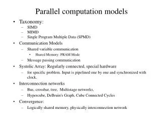
Parallel computation models. Taxonomy: SIMD MIMD Single Program Multiple Data (SPMD) Communication Models Shared variable communication Shared Memory: PRAM Mode Message passing communication Systolic Array: Regularly connected, special hardware

Parallel computation models
E N D
Presentation Transcript
Parallel computation models • Taxonomy: • SIMD • MIMD • Single Program Multiple Data (SPMD) • Communication Models • Shared variable communication • Shared Memory: PRAM Mode • Message passing communication • Systolic Array: Regularly connected, special hardware • for specific problem. Input is pipelined one by one and synchronized with clock. • Interconnection networks • Bus, crossbar, tree, Multistage networks, • Hypercube, DeBruin's Graph, Cube Connected Cycles • Convergence: • Logically shared memory, physically interconnection network
Timing Issues • Synchronous: • Every step is synchronized (central clock) • execution results predictable • PRAM is a special case • Asynchronous (no central clock) • execution results : unpredictable • example: distributed algorithms • Partially Synchronous • BSP: Bulk Synchronous Programming • LogP model: • Latency, Overhead, Gap, and P
LogP Model(Karp93) • L: upperbound on the latency incurred in sending a message of a word • o: overhead, the length of time that a PE is engaged in the transmission of • each message; during this time, the PE cannot perform other operations. • g: gap, minimum time interval between consecutive message transmissionor • reception. 1/g is per PE communication bandwidth. • P: the number of PE/memory modules. • Length W messgae: time to reach o+gW+L • process the reception: o+gW • Network has a finite capacity, at most L/g messages can be in transit from • one PE to any other PE. • Example of braodcasting 1 to n: • PRAM Concurrent Read Model: d unit of time, where d is delay of memory access • PRAM Exclusive Read Model: O(d*log_2 n) time • LogP Model: O(d*log_d n) time, d=L+o+g
CRCW model variations • Same Value (if multiple PE attempt to write, their value should be the same) • Priority (highest priority) • Random (any can be written)
Example of Shared Memory Algorithm • Adding n numbers • Max of n numbers • O(n) • O(logn) • O(1) algorithm (CRCW) 1. initially r[i] = 0, 1<= i <= n 2. for all i,j PE[i,j] read a[i] and a[j] 3. for all i,j PE[i,j] set r[i] = 1 if a[i] < a[j] 4. for all i, PE[i] do {if r[i] = 0 them max=a[i]} Applications: Boolean matrix multiplication O(1) time using O(n3) PEs
Work optimal maximum N data, P PEs • partition N data so that each PE has N/P data items. • find max of each partition • find the maximum among PEs.
Simulation of CRCW model using EREW Theorem: each step of Priority CRCW can be simulated by EREW PRAM in O(log p) steps. Proof: Each CRCW step can be simulated by a tournament (of EREW) in O(logn) time.