Download
1 / 35
350 likes | 518 Vues
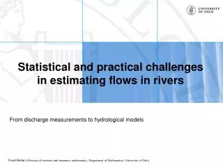
Statistical and practical challenges in estimating flows in rivers . From discharge measurements to hydrological models. Motivation. River hydrology: Management of fresh water resources Decision-making concerning flood risk and drought

E N D
Statistical and practical challenges in estimating flows in rivers From discharge measurements to hydrological models
Motivation • River hydrology: Management of fresh water resources • Decision-making concerning flood risk and drought • River hydrology => How much water is flowing through the rivers? • Key definition: discharge, Q Volume of water passing through a cross-section of the river each time unit. • Hydraulics – Mechanical properties of liquids. Assessing discharge under given physical circumstances.
Key problem 2000 • Wish: Discharge for any river location and for any point in time. • Reality: No discharge for any location or any point in time. • From B to A: • Discharges estimated from detailed measurements for specific locations and times. • Simultaneous measurements of discharge and a related quantity => relationship. Time series of related quantity => discharge time series. • Completion, ice effects. • Derived river flow quantities. • Discharge in unmeasured locations. 3/3-1908 – now 3/3-1908 – 1/1-2001 3/3-1908, 12/2-1912 13/2-1912 ….. Annual mean, 10 year flood 1980 1/1-2000 – now 1/3-2000, 23/5-2000 14/12-2000 … 5/4-2004 Annual mean, Daily 25% and 75% quantile, 10 year flood, 10 year drought 1960 1940 22/11-1910, 27/3-1939 5/2-1972 8/8-2004 27/3-1910 – now 1920 100 year flood 1/8-1972 – 31/12-1974 15/8-1972, 18/4-1973 31/10-1973 …. 1900
1) Discharge measurements and hydraulic uncertainties • Discharge estimates are often made using hydraulic knowledge and a numerical combination of several basic measurements. • De-composition of estimation errors: • Systematic contributions: method, instrument, person. • Individual contributions.
1) Discharge measurement techniques Many different methods for doing measurements that results in a discharge estimate (Herschy (1995)): • Velocity-area methods • Dilution methods • Slope-area methods
1) Velocity-area methods • Basic idea: Discharge can be de-composed into small discharge contributions throughout the cross-section. • Q(x,y)=v(x,y)xy x x+x y y y+y A x
1) Velocity-area measurements • Measure depth and velocity at several locations in a cross-section. Estimate Lambie (1978),ISO 748/3 (1997), Herschy (2002). Alternative: Acoustic velocity-area methods (ADCP) Current meter approach L2 L4 L1 L3 L5 L6 v1,1 v5,1 v2,1 v4,1 v3,1 v1,2 v5,2 v4,2 d1 v2,2 d5 v3,2 d4 d2 d3
1) Current-meter discharge estimation • Now: Numeric integration/hydraulic theory for mean velocity in each vertical. Numeric integration for each vertical contribution. Uncertainty by std. dev. tables. ISO 748/3 (1997) • Could have: Spatial statistical method incorporating hydraulic knowledge. Calibration errors: number of rotations per minute vs velocity. Creates dependencies between measurements done with the same instrument. v v8 v1 v7 v4 v2 v9 d1 d7 v6 v3 d2 d6 v5 d3 d5 rpm d4
1) Dilution methods • Release a chemical or radioactive tracer in the river. Relative concentrations downstream tells about the water flow. • For dilution of single volume: Q=V/I, where V is the released volume and I is the total relative concentration, and rc(t) is the relative concentration of the tracer downstream at time t. • Measure the downstream relative concentrations as a time series.
1) Dilution methods - challenges • Uncertainty treated only through standard error from tables or experience. ISO 9555 (1994), Day (1976). • Concentration as a process? Uncertainty of the integral. • Calibration errors. (Salt: temperature-conductivity-concentration calibration) t
1) Slope-area methods • Relationship between discharge, slope, perimeter geometry and roughness for a given water level. • Artificial discharge measurements for circumstances without proper discharge measurements. • Manning’s formula: Q(h)=(A(h)/P(h))2/3S1/2 /n, where h is the height of the water surface, S is the slope, A is the cross-section area, P is the wetted perimeter length and n is Manning’s roughness coefficient. Barnes & Davidian (1978) • Area and perimeter length: geometric measurements. P(h)=length of A(h)=Area of h
1) Slope-area challenges • Current practice: Uncertainty through standard deviations (tables)ISO 1070 (1992). • Challenge: Statistical method for estimating discharge given perimeter data + knowledge about Manning’s n. • Handle the estimation uncertainty and the dependency between slope-area ‘measurements’.
1) General discharge measurement challenges • Ideally, find f(e1, e2,…,en | s1, s2,…,sn,C,S), ei=(Qmeas-Qreal)/Qreal, si=specific data for measurement i, C=calibration data, S=knowledge of other systematic error contributions. • User friendliness in statistical hydraulic analysis. • What we have got now: f(e1, e2,…,en )=fe(e1)fe(e2)…fe(en)
2) Making discharge time series • Discharge generally expensive to measure. • Need to find a relationship between discharge and something we can measure as a time series. • Time series of related quantity + relationship to discharge Discharge time series • Most used related quantity: Stage (height of the water surface).
2) Water level and stage-discharge • Stage, h: The height of the water surface at a site in a river. Stage-discharge rating-curve h Q h0 Datum, height=0 Discharge,Q
2) Stage time series + stage-discharge relationship = discharge time series h Q Maybe the stage series itself is uncertain, too?
2) Basic properties of a stage-discharge relationship • Simple physical attributes: • Q=0 for hh0 • Q(h2)>Q(h1) for h2>h1>h0 • Parametric form suggested by hydraulics (Lambie (1978) and ISO 1100/2 (1998)): Q=C(h-h0)b • Alternatives: • Using slope-area or more detailed hydraulic modelling directly. • Q=a+b h+ c h2Yevjevich (1972),Clarke (1994) • Fenton (2001) • Neural net relationship. Supharatid (2003), Bhattacharya & Solomatine (2005) • Support Vector Machines. Sivapragasam & Muttil (2005)
2) Segmentation in stage-discharge • Q=C(h-h0)bmay be a bit too simple for some cases. • Parameters may be fixed only in stage intervals – segmentation. h h width Q
2) Fitting Q=C(h-h0)b, the old ways • Observation: Q=C(h-h0)b qlog(Q)=a+b log(h-h0) • Measure/guess h0. Fit a line manually on log-log-paper. • Measure/guess h0. Linear regression on qi vs log(hi-h0). • Plot qi vs log(hi-h0) for some plausible values of h0. Choose the h0 that makes the plot look linear. • Draw a smooth curve, fetch 3 points and calculate h0 from that. Herschy (1995) • For a host of plausible value of h0, do linear regression. Choose: h0 with least RSS. • Max likelihood on qi=a+b log(hi-h0) + i , i{1,…,n},i ~N(0,2) i.i.d.
2) Statistical challenges met for Q=C(h-h0)b Statistical model, classical estimation and asymptotic uncertainty studied by Venetis (1970). Model: qi=a+b log(hi-h0) + i , i{1,…,n}, i ~N(0,2) i.i.d. Problems discussed in Reitan & Petersen-Øverleir (2006) Alternate models: Petersen-Øverleir (2004), Moyeeda & Clark (2005). Using hydraulic knowledge - Bayesian studies: Moyeeda & Clark (2005) and Árnason (2005), Reitan & Petersen-Øverleir (2008a). Segmented curves: Petersen-Øverleir & Reitan (2005b), Reitan & Petersen-Øverleir (2008b). Measures for curve quality: curve uncertainty, trend analysis of residuals and outlier detection: Reitan & Petersen-Øverleir (2008b).
2) Challenges in error modelling Venetis (1970) model: qi=a+b log(hi-h0) + i , i ~N(0,2) can be written as Qi=Q(hi)Ei, Ei~logN(0,2), Q(h)=C(h-h0)b. For some datasets, the relative errors does not look normally distributed and/or having the same error size for all discharges? Heteroscedasticity. Residuals (estimated i‘s) for segmented analysis of station Øyreselv, 1928-1967
2) More about challenges in error modelling With uncertainty analysis from section 1 completed: Uncertainty of individual measurements and of systematic errors. With the information we have: Modelling heteroscedasticity. So far, additive models. Multiplicative error model preferable. Modelling systematic errors (small effects?). Uncertainty in stage => heteroscedasticity? ISO form not be perfect => model small-scale deviations from the curve? Ingimarsson et. al (2008) Non-normal noise / outlier detection? Denison et. al (2002)
2) Other Q=C(h-h0)b fitting challenges Ensure positive b. Not really a regression setting – stage-discharge co-variation model? Handling quality issues during fitting rather than after (different time periods). Handling slope-area data. Doing all these things in reasonable time. Prioritising Before flood After flood
2) Fitting discharge to other quantities than single stage Time dependency – changes in stage-discharge relationship can be smooth rather than abrupt. Can also explainheteroscedasticity. Dealing with hysteresis – stage + time derivative of stage. Fread (1975), Petersen-Øverleir (2006) Backwater effects – stage-fall-discharge model. El-Jabi et. al (1992), Herschy (1995), Supharatid (2003), Bhattacharya & Solomatine (2005) Index velocity method - stage-velocity-discharge model. Simpson & Bland (2000)
3) Completion Hydrological measuring stations may be inoperative for some time periods. Need to fill the missing data. Currently: Linear regression on neighbouring discharge time series. Problem: Time dependency means that the uncertainty inference from linear regression will be wrong.
3) Completion – meeting the challenge Challenge: Take the time-dependency into account and handle uncertainty concerning the filling of missing data realistically. Kalman smoother Other types of time-series models Rainfall-runoff models Ice effects – Ice affects the stage-discharge relationship. Completion or tilting the series to go through some winter measurements?Morse & Hicks (2005) Coarse time resolution - Also completion?
3) Rainfall-runoff models (lumped) Physical models of the hydrological cycle above a given point in the river. Lumped: works on spatially averaged quantities. Quantities of interest: precipitation, evaporation, storage potential and storage mechanism in surface, soil, groundwater, lakes, marshes, vegetation. Highly non-linear inference. First OLS-optimized. Statistical treatment – Clark (1973). Bayesian analysis – Kuczera (1983) P E T S0 S1 S5 S4 S2 S3 Q
4) Derived river flow quantities Discharge time series used for calculating derived quantities. Examples: mean daily discharge, total water volume for each year, expected total water volume per year, monthly 25% and 75% quantiles, the 10-year drought, the 100-year flood.
4) Flood frequency analysis T-year-flood: QT is a T-year flood if Qmax=yearly maximum discharge. Traditional: Have: Sources of uncertainty: samples variability Coles & Tawn (1996), Parent & Bernier (2003) stage-discharge errors Clarke (1999) stage time series errors Petersen-Øverleir & Reitan (2005a) completion non-stationarity
5) Filling out unmeasured areas For derived quantities: regression on catchment characteristics Upstream/downstream: scale discharge series Routing though lakes. Distributed rainfall-runoff models. Example: gridded HBV. Beldring et. al (2003) From an internal NVE presentation by Stein Beldring.
Layers Derived quantities in unmeasured areas Discharge series in unmeasured areas Meteorological estimates Hydrological parameters Derived quantities Parameters inferred from discharge sample Stage time series Completion Rating curve Individual discharge measurements Model deviances Other systematic factors Instrument calibration
Conclusions Plenty of challenges. Not only statistical but in the possibility of doing realistic statistical analysis – information flow. Awareness of uncertainty in the basic data is often lacking in the higher level analysis. Building up the foundation. User friendly combinations of statistics and programming. How much is too much? Computer resources Programming resources ISO requirements – difficult to change the procedures. Sharing of research, resources and code.
References • Árnason S (2005), Estimating nonlinear hydrological rating curves and discharge using the Bayesian approach. Masters Degree, Faculty of Engineering, University of Iceland • Barnes HH, Davidian J (1978), Indirect Methods. Hydrometry: Principles and Practices, first edition, edited by Herschy RW, John Wiley & Sons, UK • Beldring S, Engeland K, Roald LA, Sælthun NR, Voksø A (2003), Estimation of parameters in a distributed precipitation-runoff model for Norway. Hydrol Earth System Sci, 7(3): 304-316 • Bhattacharya B, Solomatine DP (2005), Neural networks and M5 model trees in modelling water level-discharge relationship, Neurocomputing, 63: 381-396 • Coles SG, Tawn JA (1996), Bayesian analysis of extreme rainfall data. Appl Stat, 45(4): 463-478 • Clarke RT (1973), A review of some mathematical models used in hydrology, with observations on their calibration and use. J Hydrol, 19:1-20 • Clarke RT (1994), Statistical modeling in hydrology. Wiley, Chichester • Clarke RT (1999), Uncertainty in the estimation of mean annual flood due to rating curve indefinition. J Hydrol, 222: 185-190 • Day TJ (1976), On the precision of salt dilution gauging. J Hydrol, 31: 293-306 • Denison DGT, Holmes CC, Mallick BK, Smith AFM (2002), Bayesian Methods for Nonlinear Classification and regression. John Wiley and Sons, New York • El-Jabi N, Wakim G, Sarraf S (1992), Stage-discharge relationship in tidal rivers. J. Waterw Port Coast Engng, ASCE, 118: 166 – 174. • Fenton JD (2001), Rating curves: Part 2 – Representation and Approximation. Conference on hydraulics in civil engineering, The Institution of Engineers, Australia, pp319-328
References Fread DL (1975), Computation of stage-discharge relationships affected by unsteady flow. Water Res Bull, 11-2: 213-228 Herschy RW (1995), Streamflow Measurement, 2nd edition. Chapman & Hall, London Herschy RW (2002), The uncertainty in a current meter measurement. Flow measurement and instrumentation, 13: 281-284 Ingimarsson KM, Hrafnkelsson B, Gardarsson SM. Snorrason A (2008), Bayesian estimation of discharge rating curves. XXV Nordic Hydrological Conference, pp. 308-317. Nordic Association for Hydrology. Reykjavik, August 11-13, 2008. ISO 748/3 (1997), Measurement of liquid flow in open channels – Velocity-area methods, Geneva ISO 1070/2 (1992), Liquid flow measurement in open channels – Slope-area method, Geneva ISO 1100/2. (1998), Stage-discharge Relation, Geneva ISO 9555/1 (1994), Measurement of liquid flow in open channels – Tracer dilution methods for the measurement of steady flow, Geneva Kuczera G (1983), Improved parameter inference in catchment models. 1. Evaluating parameter uncertainty. Water Resources Research, 19(5): 1151-1162 Lambie JC (1978), Measurement of flow - velocity-area methods. Hydrometry: Principles and Practices, first edition, edited by Herschy RW, John Wiley & Sons, UK. Morse B, Hicks F (2005), Advances in river ice hydrology 1999-2003. Hydrol Processes, 19:247-263 Moyeeda RA, Clarke RT (2005), The use of Bayesian methods for fitting rating curves, with case studies. Adv Water Res, 28:8:807-818 Parent E, Bernier J (2003), Bayesian POT modelling for historical data. J Hydrol, 274: 95-108
References Petersen-Øverleir A (2004), Accounting for heteroscedasticity in rating curve estimates. J Hydrol, 292: 173-181 Petersen-Øverleir A, Reitan T (2005a), Uncertainty in flood discharges from urban and small rural catchments due to inaccurate head determination. Nordic Hydrology 36: 245-257 Petersen-Øverleir A, Reitan T (2005b), Objective segmentation in compound rating curves. J Hydrol, 311: 188-201 Petersen-Øverleir A (2006), Modelling stage-discharge relationships affected by hysteresis using Jones formula and nonlinear regression. Hydrol Sciences, 51(3): 365-388 Reitan T, Petersen-Øverleir A (2008a), Bayesian power-law regression with a location parameter, with applications for construction of discharge rating curves. Stoc Env Res Risk Asses, 22: 351-365 Reitan T, Petersen-Øverleir A (2008b), Bayesian methods for estimating multi-segment discharge rating curves. Stoc Env Res Risk Asses, Online First Simpson MR, Bland R (2000), Methods for accurate estimation of net discharge in a tidal channel. IEEE J Oceanic Eng, 25(4): 437-445 Sivapragasam C, Muttil N (2005), Discharge rating curve extension – a new approach. Water Res Manag, 19:505-520 Supharatid S (2003), Application of a neural network model in establishing a stage-discharge relationship for a tidal river. Hydrol Processes, 17: 3085-3099 Venetis C (1970), A note on the estimation of the parameters in logarithmic stage-discharge relationships with estimation of their error, Bull Inter Assoc Sci Hydrol, 15: 105-111 Yevjevich V (1972), Stochastic processes in hydrology. Water Resources Publications, Fort Collins