Download
1 / 26
900 likes | 1.86k Vues
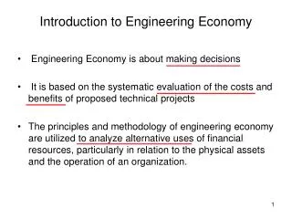
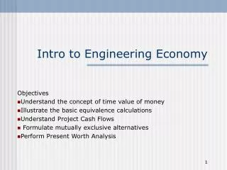
Intro to Engineering Economy. Objectives Understand the concept of time value of money Illustrate the basic equivalence calculations Understand Project Cash Flows Formulate mutually exclusive alternatives Perform Present Worth Analysis. Manufacturing. Profit. Investment. Marketing.

E N D
Intro to Engineering Economy Objectives Understand the concept of time value of money Illustrate the basic equivalence calculations Understand Project Cash Flows Formulate mutually exclusive alternatives Perform Present Worth Analysis
Manufacturing Profit Investment Marketing Engineering Economy Decisions Planning
Role of Engineering Economy • Understand the Problem • Collect all relevant data/information • Define the feasible alternatives • Evaluate each alternative • Select the “best” alternative • Implement and monitor Tools Present Worth, Future Worth Annual Worth, Rate of Return Benefit/Cost, Payback, Capitalized Cost, Value Added Major Role of Engineering Economy
Interest: The cost of money • Interest rate: a percentage that is periodically applied and added to an amount of money over a specified length of time • Interest rate for saving account • Interest rate when borrowing money • Time value of money • A dollar today is worth more than a dollar one or more years from now because of the interest (profit) it can earn • Interest is the cost of money • A cost to the borrower and an earning to the lender
Economic Equivalence • Economic Equivalence exits between cash flows that have the same economic effect and could be traded for one another in the financial market place • Cash flows can be converted to an equivalent cash flow at any point in time • Two sums of money at two different points in time can be made economically equivalent if we consider • an interest rate and, • No. of time periods between the two sums Equality in terms of Economic Value
Equivalence Illustrated $20,000 is received here • $20,000 now is not equal in magnitude to $21,800 1 year from now • But, $20,000 now is economically equivalent to $21,800 one year from now if the interest rate is 9% per year. • If you were told that the interest rate is 9%.... • Which is worth more? • $20,000 now or • $21,800 one year from now? • The two sums are economically equivalent but not numerically equal! t = 1 Yr t=0 $21,800 paid back here
Simple and Compound Interest A deposit of P dollars with interest rate of i for N periods. Simple Interest • the practice of charging an interest rate only to an initial sum (principal amount). Total interest earned is I = (iP)N Total future amount is F = P+I = P(1+iN) Compound Interest • the practice of charging an interest rate to an initial sum and to any previously accumulated interest that has not been withdrawn. Total future amount is F = P+I = P(1+i)N
P=$1,000 1 2 3 I1=$50.00 I2=$52.50 I3=$55.13 Ex: Compound Interest For compound interest, with 5% annual interest rate for 3 years Owe at t = 3 years: $1,000 + 50.00 + 52.50 + 55.13 = $1,157.63
Terminology and Symbol • P = value or amount of money at a time designated as the present or time 0. Also, P is referred to as present worth (PW), present value (PV), net present value (NPV), discounted cash flow (DCF), and capitalized cost (CC); dollars • F = value or amount of money at some future time. Also, F is called future worth (FW) and future value (FV); dollars • A = series of consecutive, equal, end‑of‑period amounts of money. Also, A is called the annual worth (AW) and equivalent uniform annual worth (EUAW); dollars per year, dollars per month • n = number of interest periods; years, months, days • i = interest rate or rate of return per time period; percent per year, percent per month • t = time, stated in periods; years, months, days, etc
Cash Flow • CASH INFLOWS • Money flowing INTO the firm from outside • Upward arrows (): • Revenues, Savings, Salvage Values, etc. • CASH OUTFLOWS • Disbursements • Downward arrows (): • First costs of assets, labor, salaries, taxes paid, utilities, rents, interest, etc. • NET CASH FLOW • two or more receipts and disbursement at the same time are summed and shown in a single arrow • Cash Inflows – Cash Outflows END-OF-PERIOD CONVENTION • placing all cash flow transactions at the end of an interest period.
Types of Cash Flows • Single cash flow • Equal (uniform) series • Linear gradient series • Geometric gradient series • Irregular series
F F 0 0 N N P P Single-Payment Factors (F/P and P/F) • Find F, given P , i, N • “Single-payment compound amount factor” F = P (1+i)N = P (F/P,i,N) • Ex: If you had $2,000 now an invested it at 10%, how much would it be worth in 8 years • Find P, given F , i , N, • “Single-payment present worth factor” P = F (1+ i )-N = F (P/F,i,N) • Ex: Suppose that $1,000 is to be received in 5 years. At an annual interest rate of 12%, what is the present worth of this amount? Also see Example 2.1 – 2.3
Example Adapted from Park (2004) A company has borrowed $250,000 to purchase an equipment. A loan was offered with 8% interest rate per year. The company plans to repay installments in equal amounts over the next 6 years. • What is annual installment? • What if the repayment is deferred for 1 year, what would be the annual installment in this case? That is, the 1st loan payment starts at the end of year 2 and continues to year 7.
0 1 2 3 4 5 6 7 8 Shifted Uniform Series • A shifted series is one whose present worth point in time is NOT t = 0. • Shifted either to the left of “0” or to the right of t = “0”. • Dealing with a uniform series: • The PW point is always one period to the left of the first series value • No matter where the series falls on the time line. i = 10% A = -$500/year P2 P0
F4 = $300 A = $500 0 1 2 3 4 5 6 7 8 F5 = -$400 Series with other single cash flow • It is common to find cash flows that are combinations of series and other single cash flows. • Solve for the series present worth values then move to t = 0. • Solve for the PW at t = 0 for the single cash flows. • Add the equivalent PW’s at t = 0. • Consider: i = 10%
Ex: Final Exam (2004) An engineering student who will soon receive his B.S. degree is considering continuing his formal education by working toward an M.S. degree. The student estimates that his average earnings for the next 6 years with a B.S. degree will be $40,000 per year. If he can get an M.S. degree in one year, his earnings should average $44,000 per year for the subsequent 5 years. His earnings while working on the M.S. degree will be negligible and his additional expenses to be paid out over this year will be $10,000. The student estimates that his average per-year earnings in the two decades following the initial 6-year period will be $42,000 and $45,000, if he does not stay for an M.S. degree. If he receives an M.S. degree his earnings per year in the two decades can be stated as $42,000 + x and $45,000 + x. The interest rate is assumed at 15%. • Draw cash flow diagrams for two options; working and studying. The diagram must be clearly labeled. • Find the value of x for which the extra investment in formal education will pay for itself. In other words, find the value of x in which the two options (working and studying) are break-even and equivalent. Note: Use up to 4 decimal points throughout your calculation.
Evaluating Alternatives • Revenue/Cost – the alternatives consist of cash inflow and cash outflows • Select the alternative with the maximum economic value • Service – the alternatives consist mainly of cost elements • Select the alternative with the minimum economic value (min. cost alternative)
Evaluating Alternatives • Independent: the decision on any one project has no effect on the decision made on another project • Mutually exclusive: Acceptance of one project will automatically rejects all other projects
Do Nothing Alt. 1 Alt. 2 Alt. m Alternatives Analysis Selection Problem Execution
Step 2: If mutually exclusive alternatives, select the highest PW alternative Step 2: If independent projects, select all project with PW 0 Evaluating Alternatives:Present Worth Analysis (PW) A process of obtaining the equivalent worth of future cash flows to some point in time – called the Present Worth (PW) At an interest rate usually equal to or greater than the Organization’s established Minimum Attractive Rate of Return (MARR). Step 1: Calculate PW of each alternative at MARR
Step 2: If mutually exclusive alternatives, select the highest PW alternative Step 2: If independent projects, select all project with PW 0 Present Worth Analysis of Equal-Life Alternatives Ex: Assume 2 investment alternatives with the same useful life of 4 years. Due to limited investment fund, the 2 alternatives are mutually exclusive. Based on the following information, which one should we select? Assume MARR = 10% Step 1: Calculate PW of each alternative at MARR Also see Ex 5.1
Ex: PW Analysis (Equal-life) Consider: Machine AMachine B First Cost $2,500 $3,500 Annual Operating Cost 900 700 Salvage Value 200 350 Life 5 years 5 years i = 10% per year Which alternative should we select?
Present Worth Analysis of Different Life Alternatives • Comparison must be made over equal time periods • Compare over the least common multiple, LCM, for their lives • Assume repeatability. Alternative will repeat the same manner over each life cycle • Cash flow estimates are the same in every life cycle • Example: {3,4, and 6} years. The lowest common life is 12 years. • Evaluate all over 12 years for a PW analysis. Also see Ex 5.2
Ex: PW Analysis (Different-life) Assume MARR 10% per year. Which alternative should we select?