Download
1 / 32
320 likes | 492 Vues
International Workshop on Multiphase and Complex Flow simulation for Industry, Cargese, October 20-24, 2003. A relaxation scheme for the numerical modelling of phase transition. Philippe Helluy , Université de Toulon , Projet SMASH, INRIA Sophia Antipolis. boiling. Introduction. Cavitation.

E N D
International Workshop on Multiphase and Complex Flow simulation for Industry, Cargese, October 20-24, 2003. A relaxation scheme for the numerical modelling of phase transition. Philippe Helluy, Université de Toulon, Projet SMASH, INRIA Sophia Antipolis.
boiling Introduction Cavitation
Introduction Demonstration
Plan • Modelling of cavitation • Non-uniqueness of the Riemann problem • Relaxation and projection finite volume scheme • Numerical results
The Euler compressible model needs a pressure law of the form The complete state law : s is the specific entropy (concave) Pressure law Caloric law Modelling Entropy and state law r : density e : internal energy But it is an incomplete law for thermal modelling (Menikoff, Plohr, 1989) T : temperature
Modelling Mixtures We consider 2 phases (with entropy functions s1 and s2) of a same simple body (liquid water and its vapor) mixed at a macroscopic scale. Entropy is an additive quantity :
Modelling Equilibrium law Mass and energy must be conserved. The equilibrium is thus determined by If the maximum is attained for 0<Y<1, we obtain (chemical potential) Generally, the maximum is attained for Y=0 or Y=1. If 0<Yeq<1, we are on the saturation curve.
Modelling Mixture law out of equilibrium Mixture pressure Mixture temperature If T1=T2, the mixture pressure law becomes (Chanteperdrix, Villedieu, Vila, 2000)
Riemann Simple model (perfect gas laws) The entropy reads Temperature equilibrium Pressure equilibrium: The fractions a and z can be eliminated
Riemann Saturation curve Out of equilibrium, we have a perfect gas law On the other side, The saturation curve is thus a line in the (T,p) plane.
Riemann Optimization with constraints Phase 2 is the most stable Phase 1 is the most stable Phases 1 and 2 are at equilibrium
Riemann Equilibrium pressure law Let We suppose (fluid (2) is heavier than fluid (1))
Riemann Shock curves Shock: Shock lagrangian velocity wL is linked to wR by a 3-shock if there is a j>0 such that: (Hugoniot curve)
Riemann Two entropy solutions On the Hugoniot curve: Menikof & Plohr, 1989 ; Jaouen 2001; …
Scheme A relaxation model for the cavitation The last equation is compatible with the second principle because, by the concavity of s (Coquel, Perthame 1998)
Scheme Relaxation-projection scheme When l=0, the previous system can be written in the classical form Finite volumes scheme (relaxation of the pressure law) Projection on the equilibrium pressure law
Scheme Numerical results
Scheme Numerical results
Scheme Numerical results
Scheme Mixture of stiffened gases Barberon, 2002 Caloric and pressure laws The mixture still satisfies a stiffened gas law Setting
Scheme Liquid High pressure (5.109Pa) Ambient pressure (105 Pa) Ambient pressure (105 Pa) 0 mm 0,08 mm wall 0,06 mm 0,015 mm 0,005 mm 200, 800, 1600, 3200 cells Convergence and CFL Tests
Scheme Convergence Tests • 200, 800, 1600, 3200 cells • convergence of the scheme Mixture density Pressure Mass Fraction
Scheme CFL Tests • Jaouen (2001) • CFL = 0.5, 0.7, 0.95 • No difference observed Mass Fraction Pressure
Results 45 cells 35 cells 10 cells 0.2 mm 12 mm IV.1 Bubble appearance • Liquid area heated at the center by a laser pulse (Andreae, Ballmann, Müller, Voss, 2002). • The laser pulse (10 MJ) increases the internal energy. • Because of the growth of the internal energy, the phase transition from liquid into a vapor – liquid mixture occurs. • Phase transition induces growth of pressure • After a few nanoseconds, • the bubble collapses. Heated liquid (1500 atm) Ambient liquid (1atm)
Results IV.1 Bubble appearance : Pressure Mixture Pressure (from 0 to 1ns)
Results IV.1 Bubble appearance : Volume Fraction Volume Fraction of Vapor (from 0 to 60ns)
Results IV.2 Bubble collapse near a rigid wall • Same example as previous test, with a rigid wall • Liquid area heated at the center by a laser pulse Wall 2.0 mm, 70 cells Heated liquid (1500 atm) 1.4 mm 0.15 mm 0.45 mm Ambient liquid (1atm) 2.4 mm, 70 cells
Results IV.2 Bubble close to a rigid wall Mixture pressure (from 0 to 2ns)
Results IV.2 Bubble close to a rigid wall Volume Fraction of Vapor (from 0 to 66ns)
Results Cavitation flowin 2D Fast projectile (1000m/s) in water (Saurel,Cocchi, Butler, 1999) final time : 225 s 15 cm, 90 cells 4 cm, 24 cells p<0 45° 2 cm Projectile 3 cm Pressure (pa)
Results Cavitation flow in 2D Fast projectile (1000m/s) in water ; final time 225 s p>0
Conclusion Conclusion • Simple method based on physics • Entropic scheme by construction • Possible extensions : reacting flows, n phases, finite reaction rate, … Perspectives • More realistic laws • Critical point