Download
1 / 172
1.75k likes | 2.14k Vues
Applied Business Forecasting and Planning. The Box-Jenkins Methodology for ARIMA Models. Introduction. Autoregressive Integrated Moving Average models (ARIMA models) were popularized by George Box and Gwilym Jenkins in the early 1970s.

E N D
Applied Business Forecasting and Planning The Box-Jenkins Methodology for ARIMA Models
Introduction • Autoregressive Integrated Moving Average models (ARIMA models) were popularized by George Box and Gwilym Jenkins in the early 1970s. • ARIMA models are a class of linear models that is capable of representing stationary as well as non-stationary time series. • ARIMA models do not involve independent variables in their construction. They make use of the information in the series itself to generate forecasts.
Introduction • ARIMA models rely heavily on autocorrelation patterns in the data. • ARIMA methodology of forecasting is different from most methods because it does not assume any particular pattern in the historical data of the series to be forecast. • It uses an interactive approach of identifying a possible model from a general class of models. The chosen model is then checked against the historical data to see if it accurately describe the series.
Introduction • Recall that, a time series data is a sequence of numerical observations naturally ordered in time • Daily closing price of IBM stock • Weekly automobile production by the Pontiac division of general Motors. • Hourly temperatures at the entrance to Grand central Station.
Introduction • Two question of paramount importance When a forecaster examines a time series data are: • Do the data exhibit a discernible pattern? • Can this be exploited to make meaningful forecasts?
Introduction • The Box-Jenkins methodology refers to a set of procedures for identifying, fitting, and checking ARIMA models with time series data.Forecasts follow directly from the form of fitted model. • The basis of BOX-Jenkins approach to modeling time series consists of three phases: • Identification • Estimation and testing • Application
Introduction • Identification • Data preparation • Transform data to stabilize variance • Differencing data to obtain stationary series • Model selection • Examine data, ACF and PACF to identify potential models
Introduction • Estimation and testing • Estimation • Estimate parameters in potential models • Select best model using suitable criterion • Diagnostics • Check ACF/PACF of residuals • Do portmanteau test of residuals • Are the residuals white noise?
Introduction • Application • Forecasting: use model to forecast
Examining correlation in time series data • The key statistic in time series analysis is the autocorrelation coefficient ( the correlation of the time series with itself, lagged 1, 2, or more periods.) • Recall the autocorrelation formula:
Examining Correlation in Time Series Data • Recall r1 indicates how successive values of Y relate to each other, r2 indicates how Y values two periods apart relate to each other, and so on. • The auto correlations at lag 1, 2, …, make up the autocorrelation function or ACF. • Autocorrelation function is a valuable tool for investigating properties of an empirical time series.
A white noise model • A white noise model is a model where observations Yt is made of two parts: a fixed value and an uncorrelated random error component. • For uncorrelated data (a time series which is white noise) we expect each autocorrelation to be close to zero. • Consider the following white noise series.
Sampling distribution of autocorrelation • The autocorrelation coefficients of white noise data have a sampling distribution that can be approximated by a normal distribution with mean zero and standard error 1/n. where n is the number of observations in the series. • This information can be used to develop tests of hypotheses and confidence intervals for ACF.
Sampling distribution of autocorrelation • For example • For our white noise series example, we expect 95% of all sample ACF to be within • If this is not the case then the series is not white noise. • The sampling distribution and standard error allow us to distinguish what is randomness or white noise from what is pattern.
Portmanteau tests • Instead of studying the ACF value one at a time, we can consider a set of them together, for example the first 10 of them (r1 through r10) all at one time. • A common test is the Box-Pierce test which is based on the Box-Pierce Q statistics • Usually h 20 is selected
Portmanteau tests • This test was originally developed by Box and Pierce for testing the residuals from a forecast model. • Any good forecast model should have forecast errors which follow a white noise model. • If the series is white noise then, the Q statistic has a chi-square distribution with (h-m) degrees of freedom, where m is the number of parameters in the model which has been fitted to the data. • The test can easily be applied to raw data, when no model has been fitted , by setting m = 0.
Example • Here is the ACF values for the white noise example.
Example • The box-Pierce Q statistics for h = 10 is • Since the data is not modeled m =0 therefore df = 10. • From table C-4 with 10 df, the probability of obtaining a chi-square value as large or larger than 5.66 is greater than 0.1. • The set of 10 rk values are not significantly different from zero.
Portmanteau tests • An alternative portmanteau test is the Ljung-Box test. • Q* has a Chi-square distribution with (h-m) degrees of freedom. • In general, the data are not white noise if the values of Q or Q* is greater than the the value given in a chi square table with = 5%.
The Partial autocorrelation coefficient • Partial autocorrelations measures the degree of association between yt and yt-k, when the effects of other time lags 1, 2, 3, …, k-1 are removed. • The partial autocorrelation coefficient of order k is evaluated by regressing yt against yt-1,…yt-k: • k (partial autocorrelation coefficient of order k) is the estimated coefficient bk.
The Partial autocorrelation coefficient • The partial autocorrelation functions (PACF) should all be close to zero for a white noise series. • If the time series is white noise, the estimated PACF are approximately independent and normally distributed with a standard error 1/n. • Therefore the same critical values of Can be used with PACF to asses if the data are white noise.
The Partial autocorrelation coefficient • It is usual to plot the partial autocorrelation function or PACF. • The PACF plot of the white noise data is presented in the next slide.
Examining stationarity of time series data • Stationarity means no growth or decline. • Data fluctuates around a constant mean independent of time and variance of the fluctuation remains constant over time. • Stationarity can be assessed using a time series plot. • Plot shows no change in the mean over time • No obvious change in the variance over time.
Examining stationarity of time series data • The autocorrelation plot can also show non-stationarity. • Significant autocorrelation for several time lags and slow decline in rk indicate non-stationarity. • The following graph shows the seasonally adjusted sales for Gap stores from 1985 to 2003.
Examining stationarity of time series data • The time series plot shows that it is non-stationary in the mean. • The next slide shows the ACF plot for this data series.
Examining stationarity of time series data • The ACF also shows a pattern typical for a non-stationary series: • Large significant ACF for the first 7 time lag • Slow decrease in the size of the autocorrelations. • The PACF is shown in the next slide.
Examining stationarity of time series data • This is also typical of a non-stationary series. • Partial autocorrelation at time lag 1 is close to one and the partial autocorrelation for the time lag 2 through 18 are close to zero.
Removing non-stationarity in time series • The non-stationary pattern in a time series data needs to be removed in order that other correlation structure present in the series can be seen before proceeding with model building. • One way of removing non-stationarity is through the method of differencing.
Removing non-stationarity in time series • The differenced series is defined as: • The following two slides shows the time series plot and the ACF plot of the monthly S&P 500 composite index from 1979 to 1997.
Removing non-stationarity in time series • The time plot shows that it is not stationary in the mean. • The ACF and PACF plot also display a pattern typical for non-stationary pattern. • Taking the first difference of the S& P 500 composite index data represents the monthly changes in the S&P 500 composite index.
Removing non-stationarity in time series • The time series plot and the ACF and PACF plots indicate that the first difference has removed the growth in the time series data. • The series looks just like a white noise with almost no autocorrelation or partial autocorrelation outside the 95% limits.
Removing non-stationarity in time series • Note that the ACF and PACF at lag 1 is outside the limits, but it is acceptable to have about 5% of spikes fall a short distance beyond the limit due to chance.
Random Walk • Let yt denote the S&P 500 composite index, then the time series plot of differenced S&P 500 composite index suggests that a suitable model for the data might be • Where et is white noise.
Random Walk • The equation in the previous slide can be rewritten as • This model is known as “random walk” model and it is widely used for non-stationary data.
Random Walk • Random walks typically have long periods of apparent trends up or down which can suddenly change direction unpredictably • They are commonly used in analyzing economic and stock price series.
Removing non-stationarity in time series • Taking first differencing is a very useful tool for removing non-statioanarity, but sometimes the differenced data will not appear stationary and it may be necessary to difference the data a second time.
Removing non-stationarity in time series • The series of second order difference is defined: • In practice, it is almost never necessary to go beyond second order differences.
Seasonal differencing • With seasonal data which is not stationary, it is appropriate to take seasonal differences. • A seasonal difference is the difference between an observation and the corresponding observation from the previous year. • Where s is the length of the season