Quantum Error Correction and Fault Tolerance
Quantum Error Correction and Fault Tolerance. Daniel Gottesman Perimeter Institute. The Classical and Quantum Worlds. Quantum Error Correction. Quantum Errors. For quantum error correction , we consider errors to be caused by a quantum channel (superoperator):. Alice. . A k A k †.

Quantum Error Correction and Fault Tolerance
E N D
Presentation Transcript
Quantum Error Correction and Fault Tolerance Daniel Gottesman Perimeter Institute
Quantum Errors For quantum error correction, we consider errors to be caused by a quantum channel (superoperator): Alice Ak Ak† Environment Bob For fault-tolerance, we must also consider errors in the gates. Examples of single-qubit errors: Bit Flip X:X0 = 1, X1 = 0 Phase Flip Z:Z0 = 0, Z1 = -1 Complete dephasing: ( + ZZ†)/2(decoherence) Rotation:R0 = 0, R1 = ei21 Frequently, we assume errors are rare, and assume at most terrors, and try to correct just that case.
QECC Conditions Theorem: A QECC can correct a set E of errors iff iEa†Ebj = Cab ij where {i} form a basis for the codewords, and Ea, Eb E. Note:The matrix Cab does not depend on i and j. As an example, consider Cab = ab. Then we can make a measurement to determine the error. space with an error Ea codespace 1 0 1 0 If Cab has rank < maximum, the code is degenerate. Otherwise, it is nondegenerate.
Linearity of QECCs Theorem:If a quantum error-correcting code (QECC) corrects errors A and B, it also corrects A + B. A general single-qubit error Ak Ak† acts like a mixture of Ak, and Ak is a 2x2 matrix. Define the Pauli group Pn on n qubits to be generated by X, Y, and Z on individual qubits. Then Pn consists of all tensor products of up to n operators I, X, Y, or Z with overall phase ±1, ±i. The weight of M Pn is the number of qubits on which M acts as a non-identity operator. The weight t Pauli operators span the space of t-qubit errors. Therefore, A QECC which correctsall weight t Paulisautomatically correctsall t-qubit errors.
Stabilizer Codes A stabilizer code is a code defined in terms of a stabilizer, a group of Pauli operators that have eigenvalue +1 for every codeword. A stabilizer S must be an Abelian subgroup of the Pauli group, and cannot contain -1, but is otherwise arbitrary. Theorem: • A stabilizer code with r generators on n qubits encodes k = n - r logical qubits. • Let N(S) = {Paulis P s.t. PM = MP M S}, and let d be the minimum weight of an element of N(S) \ S. Then the code has distance d; it corrects (d-1)/2 general errors. We say the code is a [[n, k, d]] QECC.
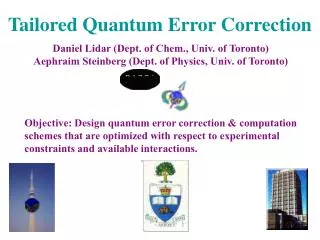
Design Goals for QECCs When we design new QECCs, there are many possible goals: • High rate (high value of both k/n and d/n). • Efficient decoding (for a general QECC, determining the exact error can take exponentially long in n). • Efficient encoding (all stabilizer codes can be encoded using O(n2) operations, but O(n) is better). • Specific error models (we can sometimes be more efficient if don’t insist on correcting all t-qubit errors). • Many symmetries (useful for fault-tolerance and sometimes other constructions). • Other application-specific properties
5-Qubit Code We can generate good codes by picking an appropriate stabilizer. For instance: X Z Z X I n = 5 physical qubits I X Z Z X [[5,1,3]] code: - 4 generators of S X I X Z Z k = 1 encoded qubit Z X I X Z Code space is { s.t. M = M S}. Distance d of this code is 3: Each single-qubit error anticommutes with a different set of generators, which determine its error syndrome. E.g.: X I I I I has syndrome 0001 I I Y I I has syndrome 1110
CSS Codes We can then define a quantum error-correcting code by choosing two classical linear codes C1 and C2, and replacing the parity check matrix of C1 with Z’s and the parity check matrix of C2 with X’s. E.g.: Z Z Z Z I I I C1: [7,4,3] Hamming Z Z I I Z Z I Z I Z I Z I Z [[7,1,3]] QECC X X X X I I I C2: [7,4,3] Hamming X X I I X X I X I X I X I X 0 0000000 + 1111000 + 1100110 + 1010101 + 0011110 + 0101101 + 0110011 + 1001011 1111111 + 0000111 + 0011001 + 0101010 + 1100001 + 1010010 + 1001100 + 0110100 1
1 1 0 - 1 1 0 - 1 0 - 1 Error Propagation When we perform multiple-qubit gates during a quantum computation, any existing errors in the computer can propagate to other qubits, even if the gate itself is perfect. CNOT propagates bit flips forward: Phase errors propagate backwards: 0 + 1 0 + 1 0 0 0 + 1 0 + 1 0 0 Of course gates can be wrong too. We assume a faulty gate can cause errors in all qubits involved in the gate. We must design protocols so that one faulty gate causes at most one error per block of the code.
Transversal Operations Error propagation is only a serious problem if it propagates errors within a block of the QECC. Then one wrong gate could cause the whole block to fail. The solution: Perform gatestransversally- i.e. only between corresponding qubits in separate blocks. 7-qubit code 7-qubit code For the 7-qubit code, we can perform CNOT, Hadamard, and R/4 (diag(1,i)) transversally. These gates generate a group of unitaries called the Clifford group.
Ancilla States However, the Clifford group is not universal (it can be efficiently simulated classically). In order to get a universal set of gates, and to perform fault-tolerant error correction, we must create special ancilla states. These ancillas are frequently (but not always) specific states encoded using the same QECC. Generally, we follow a procedure along these lines: • Use a non-FT method to create the ancilla. • Verify the ancilla carefully. This may be a very resource-intensive activity; we often imagine a separate part of the computer, an ancilla factory, is dedicated just to making ancillas. • Interact the ancilla with the data block, often using some form of teleportation.
Concatenated Codes Threshold for fault-tolerance proven using concatenated error-correcting codes. Error correction is performed more frequently at lower levels of concatenation. Effective error rate p Cp2 One qubit is encoded as n, which are encoded as n2, … (for a code correcting 1 error) If using a fault-tolerant protocol improves the error rate, apply it again and again to get the error rate as low as you like.
Threshold for Fault-Tolerance Theorem: There exists a threshold pt such that, if the error rate per gate and time step isp < pt, arbitrarily long quantum computations are possible. The physical assumptions for the theorem are discussed in the next few slides. We allow a small imperfection in every part of the quantum computer, including state preparation, gates, qubit storage, and measurement of qubits. Proof sketch: Each level of concatenation changes the effective error rate p pt (p/pt)2. The effective error rate pk after k levels of concatenation is then and for a computation of length T, we need only log (log T) levels of concatention, requiring polylog (T) extra qubits, for sufficient accuracy.
Requirements for Fault-Tolerance • Low gate error rates. • Ability to perform operations in parallel. • A way of remaining in, or returning to, the computational Hilbert space. • A source of fresh initialized qubits during the computation. • Benign error scaling: error rates that do not increase as the computer gets larger, and no large-scale correlated errors. Without some form of the following requirements, fault tolerance is impossible:
Additional Desiderata The following properties are desireable but not essential: • Ability to perform gates between distant qubits. • Fast and reliable measurement and classical computation. • Little or no error correlation (unless the registers are linked by a gate). • Very low error rates. • High parallelism. • An ample supply of extra qubits. • Even lower error rates. It is difficult, perhaps impossible, to find a physical system which satisfies all desiderata. Therefore, we need to study tradeoffs:which sets of properties will allow us to perform fault-tolerant protocols?
Threshold Values Assumptions Proof Simulation Long-range gates, many extra qubits 10-3 5 x 10⁻² Two dimensions, nearest neighbor gates 10-5 6 x 10⁻³ One dimension, two lines of qubits, nearest neighbor gates 10-6 All numbers assume probabilistic errors, good classical processing and measurement, and full parallelism. Proofs assume adversarial errors with exponential bound (errors in r specific locations have probability < pr) Simulations assume uncorrelated depolarizing channel.
Other Error Models • Coherent errors:Not serious; could add amplitudes instead of probabilities, but this worst case will not happen in practice (unproven). • Restricted types of errors:Generally not helpful; tough to design appropriate codes. (But other control techniques might help here.) • There are some exceptions: • Depolarizing channel (threshold improves somewhat) • Erasure errors (errors occur in known locations) • Pure dephasing (but must match gates to model) • Non-Markovian errors:Allowed; when the environment is weakly coupled to the system, at least for bounded system-bath Hamiltonians.
Summary • Quantum error-correcting codes exist which can correct very general types of errors on quantum systems. • A systematic theory of stabilizer codes allows us to build many interesting quantum codes. • To design fault-tolerant protocols, we must isolate errors to prevent them from spreading too far. • The threshold theorem states that we can perform arbitrarily long quantum computations provided the physical error rate is sufficiently low. • Study of the threshold value is underway, under various assumptions about the properties of the quantum computer.
Further Information • Short intro. to QECCs: quant-ph/0004072 • Short intro. to fault-tolerance: quant-ph/0701112 • Chapter 10 of Nielsen and Chuang • Chapter 7 of John Preskill’s lecture notes: http://www.theory.caltech.edu/~preskill/ph229 • Threshold proof & fault-tolerance: quant-ph/0504218 • My Ph.D. thesis: quant-ph/9705052 • Complete course on QECCs: http://perimeterinstitute.ca/personal/dgottesman/QECC2007
Quantum Error Correction Sonnet We cannot clone, perforce; instead, we split Coherence to protect it from that wrong That would destroy our valued quantum bit And make our computation take too long. Correct a flip and phase - that will suffice. If in our code another error's bred, We simply measure it, then God plays dice, Collapsing it to X or Y or Zed. We start with noisy seven, nine, or five And end with perfect one. To better spot Those flaws we must avoid, we first must strive To find which ones commute and which do not. With group and eigenstate, we've learned to fix Your quantum errors with our quantum tricks.