Download
1 / 13
160 likes | 565 Vues
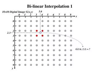
Detection of Linear and Cubic Interpolation in JPEG Compressed Images. Andrew C. Gallagher Eastman Kodak Company andrew.gallagher@kodak.com. The Problem. An image consists of a number of discrete samples. Interpolation can be used to modify the number of and locations of the samples.

E N D
Detection of Linear and Cubic Interpolation in JPEG Compressed Images Andrew C. Gallagher Eastman Kodak Company andrew.gallagher@kodak.com Andrew C. Gallagher 1 CRV2005
The Problem • An image consists of a number of discrete samples. • Interpolation can be used to modify the number of and locations of the samples. • Given an image, can interpolation be detected? If so, can the interpolation rate be determined? Andrew C. Gallagher 2 CRV2005
The Concept i(x0) y(n0) y(n1) y(n2) • A interpolated sample is a linear combination of neighboring original samples y(n0). • The weights depend on the relative positions of the original and interpolated samples. • Thus, the distribution (calculated from many lines) of interpolated samples depends on position. x0 n0 n1 n2 Original samples and an interpolated sample Andrew C. Gallagher 3 CRV2005
The Periodic Signal v(x) i(x0 -D) i(x0 -D) i(x0) y(n0) y(n1) y(n2) • The second derivative of interpolated samples is computed. • The distribution of the resulting signal is periodic with period equal to the period of the original signal. • The expected periodic signal can be calculated explicitly for specific interpolators, assuming the sample value distribution is known. d x0-D x0 x0+D n0 n1 n2 Original samples and an interpolated sample 1 period v(x) n0 n1 n2 Distribution (standard deviation) of interpolated samples Andrew C. Gallagher 4 CRV2005
The Periodic Signal v(x) • Linear Interpolation • Cubic Interpolation This property can be exploited by an algorithm designed to detect linear interpolation. Andrew C. Gallagher 5 CRV2005
The Algorithm p(i,j) • In Matlab, the first three boxes can be executed as: • bdd =diff(diff(double(b))); • bm = mean(abs(bdd),2); • bf = fft(bm); • A peak in the DFT signal corresponds to interpolation with rate compute second derivativeof each row average across rows compute Discrete Fourier Transform estimate interpolation rate N (assuming no aliasing) Andrew C. Gallagher 6 CRV2005
Resolving Aliasing • The algorithm produces samples of the periodic signal v(x). • Aliasing occurs when sampled below the Nyquist rate (2 samples per period). • All interpolation rateswill alias to N. • Only two possible solutions for rates N>1 (upsampling). An infinite number of solutions for N<1. • The correct rate can often be determined through prior knowledge of the system. (Q a positive integer) Andrew C. Gallagher 7 CRV2005
Example Signals: N = 2 After computing DFT After summing across rows v(x) Andrew C. Gallagher 8 CRV2005
Example DFT Signals Andrew C. Gallagher 9 CRV2005
Effect of JPEG Compression • Heavy JPEG compression appears similar to an interpolation by 8. • Therefore, the peaks in the DFT signal associated with JPEG compression must be ignored. interpolation N = 2.8JPEG compression no interpolationJPEG compression o(i,j) digital zoom by N After computing DFT JPEG compression p(i,j) Andrew C. Gallagher 10 CRV2005
Experiment • A Kodak CX7300 (3MP) captured 114 images • 13 images were non-interpolated. The remainder were interpolated with rate between 1.1 and 3.0. N Andrew C. Gallagher 11 CRV2005
Results • Algorithm correctly classified between interpolated (101) and non-interpolated (13) images. • Interpolation rate was correctly estimated for 85 images. • For the remaining 16 images, the algorithm identified the interpolation rate as either 1.5 or 3.0. This is correct but ambiguous. Andrew C. Gallagher 12 CRV2005
Conclusions • Linear interpolation in images can be robustly detected. • The interpolation detection algorithm performs well even when the interpolated image has undergone JPEG compression. • The algorithm is computationally efficient. • The algorithm has commercial applications in printing, image metrology and authentication. Andrew C. Gallagher 13 CRV2005