Quick-Sort
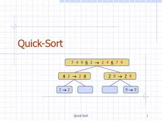
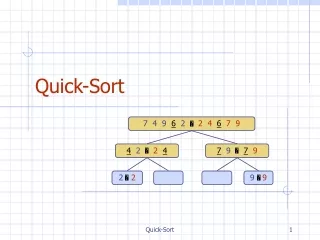
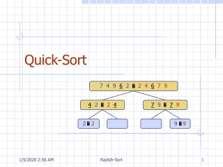
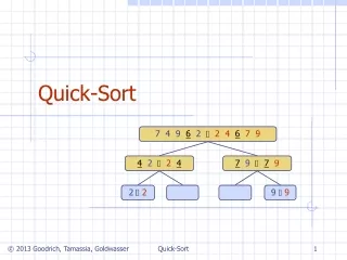
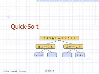
7 4 9 6 2 2 4 6 7 9. 4 2 2 4. 7 9 7 9. 2 2. 9 9. Quick-Sort. Quick-sort is a randomized sorting algorithm based on the divide-and-conquer paradigm: Divide : pick a random element x (called pivot ) and partition S into L elements less than x

Quick-Sort
E N D
Presentation Transcript
7 4 9 6 2 2 4 6 7 9 4 2 2 4 7 9 7 9 2 2 9 9 Quick-Sort Quick-Sort
Quick-sort is a randomized sorting algorithm based on the divide-and-conquer paradigm: Divide: pick a random element x (called pivot) and partition S into L elements less than x E elements equal x G elements greater than x Recur: sort L and G Conquer: join L, Eand G Quick-Sort (§ 10.2) x x L G E x Quick-Sort
Partition Algorithmpartition(S,p) Inputsequence S, position p of pivot Outputsubsequences L,E, G of the elements of S less than, equal to, or greater than the pivot, resp. L,E, G empty sequences x S.remove(p) whileS.isEmpty() y S.remove(S.first()) ify<x L.insertLast(y) else if y=x E.insertLast(y) else{ y > x } G.insertLast(y) return L,E, G • We partition an input sequence as follows: • We remove, in turn, each element y from S and • We insert y into L, Eor G,depending on the result of the comparison with the pivot x • Each insertion and removal is at the beginning or at the end of a sequence, and hence takes O(1) time • Thus, the partition step of quick-sort takes O(n) time Quick-Sort
Quick-Sort Tree • An execution of quick-sort is depicted by a binary tree • Each node represents a recursive call of quick-sort and stores: • Unsorted sequence before the execution and its pivot • Sorted sequence at the end of the execution • The root is the initial call • The leaves are calls on subsequences of size 0 or 1 7 4 9 6 2 2 4 6 7 9 4 2 2 4 7 9 7 9 2 2 9 9 Quick-Sort
Execution Example • Pivot selection 7 2 9 4 3 7 6 11 2 3 4 6 7 8 9 7 2 9 4 2 4 7 9 3 8 6 1 1 3 8 6 9 4 4 9 3 3 8 8 2 2 9 9 4 4 Quick-Sort
Execution Example (cont.) • Partition, recursive call, pivot selection 7 2 9 4 3 7 6 11 2 3 4 6 7 8 9 2 4 3 1 2 4 7 9 3 8 6 1 1 3 8 6 9 4 4 9 3 3 8 8 2 2 9 9 4 4 Quick-Sort
Execution Example (cont.) • Partition, recursive call, base case 7 2 9 4 3 7 6 11 2 3 4 6 7 8 9 2 4 3 1 2 4 7 3 8 6 1 1 3 8 6 11 9 4 4 9 3 3 8 8 9 9 4 4 Quick-Sort
Execution Example (cont.) • Recursive call, …, base case, join 7 2 9 4 3 7 6 11 2 3 4 6 7 8 9 2 4 3 1 1 2 3 4 3 8 6 1 1 3 8 6 11 4 334 3 3 8 8 9 9 44 Quick-Sort
Execution Example (cont.) • Recursive call, pivot selection 7 2 9 4 3 7 6 11 2 3 4 6 7 8 9 2 4 3 1 1 2 3 4 7 9 7 1 1 3 8 6 11 4 334 8 8 9 9 9 9 44 Quick-Sort
Execution Example (cont.) • Partition, …, recursive call, base case 7 2 9 4 3 7 6 11 2 3 4 6 7 8 9 2 4 3 1 1 2 3 4 7 9 7 1 1 3 8 6 11 4 334 8 8 99 9 9 44 Quick-Sort
Execution Example (cont.) • Join, join 7 2 9 4 3 7 6 1 1 2 3 4 67 7 9 2 4 3 1 1 2 3 4 7 9 7 1779 11 4 334 8 8 99 9 9 44 Quick-Sort
Worst-case Running Time • The worst case for quick-sort occurs when the pivot is the unique minimum or maximum element • One of L and G has size n - 1 and the other has size 0 • The running time is proportional to the sum n+ (n- 1) + … + 2 + 1 • Thus, the worst-case running time of quick-sort is O(n2) … Quick-Sort
Consider a recursive call of quick-sort on a sequence of size s Good call: the sizes of L and G are each less than 3s/4 Bad call: one of L and G has size greater than 3s/4 A call is good with probability 1/2 1/2 of the possible pivots cause good calls: 1 2 3 4 5 6 7 8 9 10 11 12 13 14 15 16 Expected Running Time 7 2 9 4 3 7 6 1 9 7 2 9 4 3 7 6 1 1 7 2 9 4 3 7 6 2 4 3 1 7 9 7 1 1 Good call Bad call Bad pivots Good pivots Bad pivots Quick-Sort
The expected height of the quick-sort tree is O(log n) The amount or work done at the nodes of the same depth is O(n) Thus, the expected running time of quick-sort is O(n log n) Expected Running Time, Part 2 Quick-Sort
Summary of Sorting Algorithms Quick-Sort
Comparison with other sort algorithms Although heapsort has the same time bounds as mergesort, it requires only Ω(1) auxiliary space instead of mergesort's Ω(n), and is consequently often faster in practical implementations. Quicksort, however, is considered by many to be the fastest general-purpose sort algorithm in practice. Its average-case complexity is O(n log n), with a much smaller coefficient, in good implementations, than mergesort's, even though it is quadratic in the worst case. On the plus side, mergesort is a stable sort, parallelizes better, and is more efficient at handling slow-to-access sequential media. Mergesort is often the best choice for sorting a linked list: in this situation it is relatively easy to implement a merge sort in such a way that it does not require Ω(n) auxiliary space (instead only Ω(1)), and the slow random-access performance of a linked list makes some other algorithms (such as quick sort) perform poorly, and others (such as heapsort) completely impossible. As of Perl 5.8, mergesort is its default sorting algorithm (it was quicksort in previous versions of Perl). In Java, the Arrays.sort() methods use mergesort and a tuned quicksort depending on the datatypes. en.wikipedia.org/wiki/Merge_sort