Download
1 / 22
220 likes | 252 Vues
Learn how to solve Linear Programming problems using the graphical method step by step. Understand the feasible region and optimize the objective function to find an optimal solution.

E N D
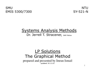
SMU EMIS 8374 LP Solutions The Graphical Method prepared by Imran Ismail updated 19 January 2006
Consider the following LP Maximize X + 2Y Subject to: X + Y 4 X - 2Y 2 -2X + Y 2 X, Y 0 This problem is in two dimensions and can be solved graphically.
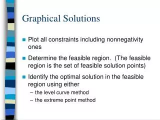
Finding the Feasible Region We begin by graphing the constraints on an XY coordinate system to determine the set of all points that satisfy all the constraints. This set of points is known as the feasible region for the LP. Since both variables must be non-negative, we know that the feasible region must be within the first quadrant.
The set of solutions to the equation X + Y = 4 can be represented by the straight line passing through the points (4,0) and (0,4) in the XY plane. The shaded triangle below represents the set of points satisfying the constraint X + Y 4, X 0, Y 0.
And for constraint 3, -2X+Y 2: Since X and Y must be nonnegative, the feasible region for the LP is the bounded by the three lines described (and shown) above and the X and Y axes. Any point inside or on the boundary of the region described above is a feasible solution to the LP.
Finding an Optimal Solution The objective function is given as an equation whose value has yet to be determined. The information provided in the LP gives us two clues: • The function has to be maximized • The function must satisfy all constraints i.e. it must lie in the feasible regions
In such an instance, we can start by assuming an objective function value of 0 (zero). This gives us the following equation X + 2Y = 0 The line above will provide us with a set of points that will have an objective function value of 0. When drawn on the graph, the segment of this line that intersects the feasible region will represent the set of feasible solutions with an objective function value of zero. In this case, the set is just the single point (0,0).
Similarly, the line X + 2Y = 2 describes the set of points that have an objective function value of two. So, the segment of this line that intersects the feasible region represents the set of feasible solutions with an objective function value of two. We can continue this method till we reach an objective function value such that it no longer intersects the feasible region.
By continuing on in this fashion, we can find an optimal solution for the LP by "pushing" the objective function line up until it last touches the feasible region.
This occurs when we graph the line X + 2Y = 22/3 = 7.333 which intersects the feasible region at the point (2/3, 10/3). Since there are no feasible solutions with a greater objective function value than 22/3, we say that X = 2/3, Y = 10/3 is an optimal solution and that 22/3 is the optimal value for the objective function.
It is important to investigate how other objective functions might behave given the same feasible region.
The “Brute Force” Method Using the fact that if an LP has an optimal solution, then it has an extreme point solution, we can use a "brute force" method to find an optimal solution by: testing each extreme point to see if it is feasible and then comparing the objective function values. Recall that an extreme, or corner-point, solution is formed by the intersection of two of the constraints.
In our example we can identify the extreme points by labeling them A, B, C, D and E, as shown below. A E B D C
Point A is formed by the intersection of: X + Y = 4 and –2X + Y = 2 and similarly: B: X - 2Y = 2 and X + Y = 4 C: X - 2Y = 2 and Y = 0 D: X = 0 and Y = 0 E: -2X + Y = 2 and X = 0 Solving these equations and plugging them into the objective function, we can calculate the objective function value all of the extreme points of the feasible region.
The co-ordinate points of A give us the maximum objective function value.
Conclusion The graphical method and the brute force method will always obtain the same result. In our example, it was found that the optimal solution is such that: • Xopt=2/3 = 0.66 • Yopt=10/3 = 3.33 • Zopt = 22/3 = 7.333
Other Special Cases of LP • Adding the constraint Y 4 to the original LP makes the problem infeasible. • Removing the constraint X + Y 4from the original LP makes the problem unbounded. • Changing the objective function of the original LP to gives an LP with multiple optimal solutions.