Gravitational Waves and the R-modes
430 likes | 674 Vues
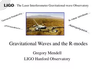
: The Laser Interferometer Gravitational-wave Observatory. Gravitational Waves and the R-modes. Gregory Mendell LIGO Hanford Observatory. Who’s Involved?. Caltech, MIT, and the LIGO Science Collaboration. Sponsored by the National Science Foundation. The Observatories. LIGO Hanford.

Gravitational Waves and the R-modes
E N D
Presentation Transcript
: The Laser Interferometer Gravitational-wave Observatory Gravitational Waves and the R-modes Gregory Mendell LIGO Hanford Observatory
Who’s Involved? Caltech, MIT, and the LIGO Science Collaboration Sponsored by the National Science Foundation
The Observatories LIGO Hanford LIGO Livingston Photos: http:// www.ligo.caltech.edu; http://www.ligo-la.caltech.edu
Gravitational Waves • Gravitation = spacetime curvature described by the metric tensor: • Weak Field Limit: • TT Gauge:
Gravitational-wave Strain D. Sigg LIGO-P980007-00-D
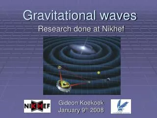
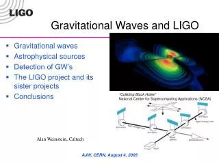
How Does LIGO Work? Gravitational-wave Strain: LIGO is an “ear” on the universe, listening for cosmic spacetime vibrations. LIGO is a lab looking for GW’s. Figures: K. S. Thorne gr-qc/9704042; D. Sigg LIGO-P980007-00-D
LMXBs Astrophysical Sources Pulsars Black Holes Stochastic Background Supernovae Photos: http://antwrp.gsfc.nasa.gov; http://imagine.gsfc.nasa.gov
“Newtonian” quadrupole formula. • Stochastic (limit GW; cosmic strings; BH from massive pop III stars: h = 10-23 – 10-21) • Burst (SN at distance of Virgo Cluster: h = 10-23 – 10-21; rate = 1/yr) • Inspiral (hmax = 10-22 for NS-NS@ 200 Mpc; rate = 3/yr; NS-BH; BH-BH) • Periodic (h = 10-25 for 10 ms pulsar with maximum ellipticity at 1 Kpc; h = 10-27 for 2 ms LMXB in equilibrium at 1 Kpc) Reviews: K. S. Thorne 100 Yrs of Gravitation; P. R. Saulson, Fund. of Interferometric GW Detectors
Noise Curves Figure: D. Sigg LIGO-P980007-00-D
Signal to Noise Ratio • h = signal amplitude • T = observation time or duration of signal or period of the characteristic frequency of the signal. • n2 = power spectrum of the noise
Sensitivity Curves Figure: Brady ITP seminar summer 2000
Known Possible Periodic Sources • Are neutron stars: the sun compress to size of city. Compact (2GM/Rc2 ~ .2) and ultra dense (1014 g/cm3). • Are composed of (superfluid) neutrons, (superconducting) protons, electrons, + exotic particles (e.g., hyperons) or strange stars composed of an even more exotic up, down, and strange quark soup. • Spin Rapidly (~ .1 Hz to 642 Hz i.e., within the LIGO band.) LMXBs
Neutron (Strange) Star Models solid crust Fe, etc. up down n e- p+ strange n p+ dissipative boundary layer quark soup fluid interior Courtesy Justin Kinney
Periodic sources emit GWs due to… • Rotation about nonsymmetry axis • Strain induced asymmetry: • Accretion induced emission • Unstable oscillation modes
GR tends to drive all rotating stars unstable! Internal dissipation suppresses the instability in all but very compact stars. Gravitational-radiation Driven Instability of Rotating Stars
Ocean Wave Instability Wind Current
Perturbations in Rotating Neutron Stars • Neutron star rotates with angular velocity > 0. • Some type of “wave” perturbation flows in opposite direction with phase velocity /m, as seen in rotating frame of star. • Perturbations create rotating mass and momentum multipoles, which emit GR. Rotating neutron star. /m Perturbations in rotating frame. Courtesy Justin Kinney
GR Causes Instability • If - /m > 0, star “drags” perturbations in opposite direction. • GR caries away positive angular momentum. • This adds negative angular momentum to the perturbations. • This increases their amplitude! - /m Star drags perturbations in opposite direction. GR drives mode instability. Courtesy Justin Kinney
The R-modes • The r-modes corresponds to oscillating flows of material (currents) in the star that arise due to the Coriolis effect. The r-mode frequency is proportional to the angular velocity, . • The current pattern travels in the azimuthal direction around the star as exp(it + im) • For the m = 2 r-mode: • Phase velocity in the corotating frame: -1/3 • Phase velocity in the inertial frame: +2/3
R-mode Instability Calculations • Gravitation radiation tends to make the r-modes grow on a time scale GR • Internal friction (e.g., viscosity) in the star tends to damp the r-modes on a time scale F • The shorter time scale wins: • GRF : Unstable! • GR F: Stable!
Key Parameters to Understanding the R-mode Instability • Critical angular velocity for the onset of the instability • Saturation amplitude
MVBL Critical Angular Velocity B = 1012 B = 1011 B = 1010 B = 0 Mendell 2001, Phys Rev D64 044009; gr-qc/0102042
R-mode Movie See: http://www.cacr.caltech.edu/projects/hydrligo/rmode.html Lee Lindblom, Joel E. Tohline and Michele Vallisneri (2001), Phys. Rev. Letters 86, 1152-1155 (2001). R-modes in newborn NS are saturated by breaking waves. Computed using Fortran 90 code linked wtih the MPI library on CACR’s HP Exemplar V2500. Owen and Lindblom gr-qc/0111024: r-modes produce 100 s burst with f ~ 940-980 Hz and optimal SNR ~ 1.2-12 for r = 20 Mpc and enhanced LIGO.
Basic Detection Strategy • Coherently add the signal • Signal to noise ratio ~ sqrt(T) • Can always win as long as • Sum stays coherent • Understand the noise • Do not exceed computational limits
Amplitude Modulation Figure: D. Sigg LIGO-P980007-00-D
Phase Modulation • The phase is modulated by the intrinsic frequency evolution of the source and by the Doppler effect due to the Earth’s motion • The Doppler effect can be ignored for
DeFT Algorithm AEI: Schutz & Papa gr-qc/9905018; Williams and Schutz gr-qc/9912029; Berukoff and Papa LAL Documentation
Advantages of DeFT Code • Pkb is peaked. Can sum over only 16 k’s • Complexity reduced from O(MN number of phase models) to O(MNlog2N + M number of phase models). • Unfortunately, number phase models increased by factor of M/log2MN over FFT of modulated data. FFT is O(MNlog2MN number of phase models/MN.) • But memory requirements much less than FFT, and easy to divide DeFT code into frequency bands and run on parallel computing cluster. • Need 1010 – 1020 phase models, depending on frequency band & number of spin down parameters, for no more than 30% power loss due to mismatch.
Basic Confidence Limit • Probability stationary white noise will result in power greater than or equal to Pf: • Threshold needed so that probability of false detection = 1 – . Brady, Creighton, Cutler, Schutz gr-qc/9702050.
Maximum Likehood Estimator Jaranowski, Krolak, Schutz gr-qc/9804014.
LDAS Hardware 14.5 TB Disk Cache Beowulf Cluster