Molecular dynamics

1. Molecular dynamics ECE 697S: Topics in Computational Biology Naomi Fox March 13, 2006

2. Outline • Why simulate motion of molecules? • Energy model of conformation • Two main approaches: • Monte Carlo - stochastic • Molecular dynamics - deterministic • Applications of MD • Speeding up MD

3. Why simulate motion? • Predict structure • Understand interactions • Understand properties • Learn about normal modes of vibration • Design of bio-nano materials • Experiment on what cannot be studied experimentally • Obtain a movie of the interacting molecules

4. Structure implies function • central dogma: sequence to structure • After protein is generated, it folds without the help of external agents (except solvent) • Difficult problem for humans to predict 3-d structure from 1-d protein sequence • Organic chemists know how structure implies function for small molecular systems. Proteins are much larger, and more difficult. Open problem. central dogma

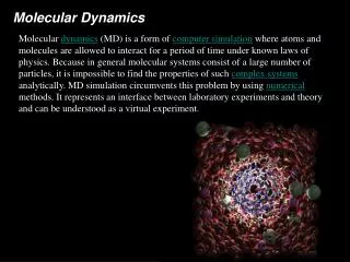
5. Aquaporin simulation 2004 Winner of Visualization Challenge in Science and Engineering, Organized by the National Science Foundation and Science Magazine.

6. Aquaporin simulation Structure, Dynamics, and Function of Aquaporins http://www.ks.uiuc.edu/Research/aquaporins/

7. Method of Molecular Dynamics • Use physics to find the potential energy between all pairs of atoms. • Move atoms to the next state. • Repeat.

8. Energy Function • Target function that MD tries to optimize • Describes the interaction energies of all atoms and molecules in the system • Always an approximation • Closer to real physics --> more realistic, more computation time (I.e. smaller time steps and more interactions increase accuracy)

9. Scale in Simulations Hy = Ey continuum mesoscale Monte Carlo Time Scale 10-6 S molecular dynamics domain 10-8 S quantum D exp(- E/kT) chemistry 10-12 S F = MA 10-10 M 10-8 M 10-6 M 10-4 M Length Scale Taken from Grant D. Smith Department of Materials Science and Engineering Department of Chemical and Fuels Engineering University of Utah http://www.che.utah.edu/~gdsmith/tutorials/tutorial1.ppt

10. The energy model • Proposed by Linus Pauling in the 1930s • Bond angles and lengths are almost always the same • Energy model broken up into two parts: • Covalent terms • Bond distances (1-2 interactions) • Bond angles (1-3) • Dihedral angles (1-4) • Non-covalent terms • Forces at a distance between all non-bonded atoms http://cmm.cit.nih.gov/modeling/guide_documents/molecular_mechanics_document.html The NIH Guide to Molecular Modeling

11. The energy equation Energy = Stretching Energy + Bending Energy + Torsion Energy + Non-Bonded Interaction Energy These equations together with the data (parameters) required to describe the behavior of different kinds of atoms and bonds, is called a force-field.

12. Bond Stretching Energy kb is the spring constant of the bond. r0 is the bond length at equilibrium. Unique kb and r0 assigned for each bond pair, i.e. C-C, O-H

13. Bending Energy k is the spring constant of the bend. 0 is the bond length at equilibrium. Unique parameters for angle bending are assigned to each bonded triplet of atoms based on their types (e.g. C-C-C, C-O-C, C-C-H, etc.)

14. The “Hookeian” potential kb and k broaden or steepen the slope of the parabola. The larger the value of k, the more energy is required to deform an angle (or bond) from its equilibrium value.

15. Torsion Energy The parameters are determined from curve fitting. Unique parameters for torsional rotation are assigned to each bonded quartet of atoms based on their types (e.g. C-C-C-C, C-O-C-N, H-C-C-H, etc.) • A controls the amplitude of the curve • n controls its periodicity • shifts the entire curve along the rotation angle axis ().

16. Torsion Energy parameters A is the amplitude. n reflects the type symmetry in the dihedral angle.  used to synchronize the torsional potential to the initial rotameric state of the molecule

17. Non-bonded Energy A determines the degree the attractiveness B determines the degree of repulsion q is the charge A determines the degree the attractiveness B determines the degree of repulsion q is the charge

18. Non-bonded Energy parameters

19. Stochastic method aka Monte Carlo Deterministic method aka Molecular Dynamics (some ambiguity of how term is used) Energy Model in Action Goal: energy minimization

20. Simulating In A Solvent • The smaller the system, the more particles on the surface • 1000 atom cubic crystal, 49% on surface • 10^6 atom cubic crystal, 6% on surface • Would like to simulate infinite bulk surrounding N-particle system • Two approaches: • Implicitly • Explicitly • Ex. Periodic boundary conditions Schematic representation of periodic boundary conditions. http://www.ccl.net/cca/documents/molecular-modeling/node9.html

21. Monte Carlo Explore the energy surface by randomly probing the configuration space Metropolis method (avoids local minima): • Specify the initial atom coordinates. • Select atom i randomly and move it by random displacement. • Calculate the change of potential energy, E corresponding to this displacement. • If E < 0, accept the new coordinates and go to step 2. • Otherwise, if E  0, select a random R in the range [0,1] and: • If e-E/kT < R accept and go to step 2 • If e-E/kT R reject and go to step 2

22. Properties of MC simulation • System behaves as a Markov process • Current state depends only on previous. • Converges quickly. • System is ergodic (any state can be reached from any other state). • Accepted more by physicists than by chemists. • Not deterministic and does not offer time evolution of the system.

23. Deterministic Approach • Provides us with a trajectory of the system. • Typical simulations of small proteins including surrounding solvent in the pico-seconds.

24. Deterministic / MD methodology • From atom positions, velocities, and accelerations, calculate atom positions and velocities at the next time step. • Integrating these infinitesimal steps yields the trajectory of the system for any desired time range. • There are efficient methods for integrating these elementary steps with Verlet and leapfrog algorithms being the most commonly used.

25. MD algorithm {r(t+Dt), v(t+Dt)} {r(t), v(t)} • Initialize system • Ensure particles do not overlap in initial positions (can use lattice) • Randomly assign velocities. • Move and integrate. Leapfrog algorithm

26. Paper: The role of molecular modeling in bionanotechnology • Molecular modeling for r+d of bionanotechnology • Three case studies: • Polarizability of carbon nanotubes • Nanopores for DNA sequencing • Nanodiscs for experimenting on membrane proteins

27. Case study 1:Towards an efficient description of carbon nanotube-biomolecule interaction • Single-walled carbon nanotubes (SWNT) can be used for in vivo biosensor applications. • SWNTs are highly-polarizable • Used MD to develop accurate description of the influence of biomolecules on nanotube electronic properties. • Furnishes ability to test nanotube electronic properties in realistic biological environments.

28. Polarizable SWNT model • Studied water-nanotube and ion-nanotube interactions. • Engineers seek to control the transport of ions or charged molecules through SWNTs by means of external electric fields. (a) Top view (b) side view of an ideal 12-section SWNT. © Potential energy profiles for same SWNT interacting with a water molecule of fixed orientation at various positions along tube axis.

29. Case study 2:Nanopore device for high-throughput sequencing of DNA • With current technology, individual genomes determined to 99.99% accuracy within 2 months for 10 million dollars. • Describes a device that may provide alternative

30. Nanopore device • 2-nm-diameter pore in a 2-5nm thick synthetic membrane. • Sequence of a DNA molecule can be read by such a device through a semiconductor detector in the pore • A,C,G, and T nucleotides differ by only a few atoms • Essential to characterize conformation of DNA inside the pore in atomic detail

31. Typical translocation event • A 1.4V bias applied to membrane. • 20 base-pair fragment of double stranded DNA placed in front of a nanopore. • End of DNA nearest to the pore is pulled into the pore by its charged backbone (a,b) • System reaches a meta-stable state (c) and translocation halts. • Base pairs start to split. Some freed nucleotides adhere to pore surface. • Voltage increased momentarily to drive system out of metastable state. • DNA exits pore. One of the bases holds firmly to the pore surface. • After 50ns, most of DNA has left pore. Nine of twenty base pairs are split.

32. Case study 3:Nanodiscs: discoidal protein-lipid particles • Nanodiscs provide a platform in which to embed, solubilize, and study single membrane proteins. • Membrane proteins are difficult to study experimentally. • Often studied under non-native conditions, with artifacts unknown.

33. MD simulation of assembly of nanodiscs • Using an optimized starting ratio of protein to lipid, homogeneous nanodiscs form with discrete size and composition. • Predict structure of nandodiscs by simulating the experimental self-assembly. • To account for full process, used Marrink et-al coarse-grained lipid-water model. • Protein amino acid residues are represented by 2 beads • DPPC lipids represented by 12 beads. • 4 water molecules are represented 1 bead.

34. Conclusions • Protein folds from 10 to 100s of s. Longest simulations ~1 s. • Can we speed up MD? • Would like: • larger systems • longer runs • more trajectories • approaches: • Mix in experimental data • Steered MD • Massive parallel computation • Course-grained methods Steered MD example Bacteriorhodopsin Steered molecular dynamics, performed by applying a series of external forces to retinal, allow one to extract retinal from bR once the Schiff base bond to Lys216 is cleaved

35. Future of MD • Review of deterministic method for molecular dynamics • Two examples of approaches for making MD ‘faster’ • Questions

36. MD algorithm • Initialize system • Ensure particles do not overlap in initial positions (can use lattice) • Randomly assign velocities. • Compute Energy Etotal = Ebond + Etorsion + Ebond-angle + Enon-bond • Get velocities of atoms, then move for timestep (~1fs) {r(t+Dt), v(t+Dt)} {r(t), v(t)}

37. Two example approaches to speeding up molecular simulation • Collect large number of trajectories using traditional MD, and see if folding rates agree with lab results. • Exploit geometry of the system to remove number of nodes that must be considered.

38. Paper: Absolute comparison of simulated and experimental protein-folding dynamics • Statistically compared computational predictions and experimentally determined mean folding times for small protein (BBA5). • Used massively distributed cluster to accumulate thousands of 5 to 20 ns trajectories. • Found computational predictions in excellent agreement with experimentally determined mean folding times and equilibrium times.

39. Similar to SETI@home, volunteers run screensaver software to donate unused CPU cycles. • Since October 1, 2000, over 1,000,000 CPUs throughout the world have participated in Folding@Home.

40. Approach to simulation • Simulated two BBA5 mutants • Considered fast-folding, mean folding time 10 s • 23 residues • Has -hairpin turn and -helix motif • Statistically, 10 out of 10,000 molecules will be folded after 10 ns. • Qualitatively reasonable but arbitrary criteria used to discriminate folded structures. • Each final conformation aligned to C positions of low energy BBA5 NMR structure and calculated r.m.s.d. • A conformation was folded if it had the helix, hairpin, and low r.m.s.d.C

41. Results • Acquired a total of 32500 trajectories • Observed -hairpin in 1100 trajectories • Observed -helix in 21000 trajectories • Of 9000 double-mutant trajectories, 16 were folded after 20ns.

42. Results

43. Limitations • Criteria for discrimination of folded structures is arbitrary • Does not represent structure prediction, because relies on C positions of BBA5 • Native state flexibility may be indication that force field is insufficiently accurate • Experimental folding rate uncertainty large (instrument latencies)

44. Conclusions • Contributes to body of knowledge about rapid protein dynamics. • Found following consistent between simulation and experimental evidence : • Helical structure in the unfolded state • Rate of helix formation • Rate of hairpin formation • Rate for folding • “The ability to investigate directly folding dynamics and heterogeneity with molecular dynamics will bring molecular dynamics to the same prominence in protein folding that it has already achieved in structural modeling.”

45. Paper: Constrained geometric simulation of diffusive motion in proteins • Old method • MD considers all 3N degrees of motion • Accurate trajectories for atoms only obtained with short time step (~femtosecond) • 10ns requires weeks of CPU time to compute • Most biologically relevant motions take place on milliseconds to seconds timescale • New method • Geometric simulation for proteins

46. Differs from MD • Not time-dependent, but distance dependent • Obtain collections of possible conformations, which define a trajectory that respects stereo-chemistry • Measure of the progression of motion is distance rather than time: • Mobility is monitored by RMSD from a reference conformer.

47. Two components to geometric simulation • FIRST - Find which regions are rigid and which are flexible • FRODA - generate sterically accurate motions of a protein using rigidity information

48. FIRST • Floppy Inclusion and Rigid Substructure Topography • Given a structure (graph of atoms and covalent bonds), identify rigid and flexible regions

49. FRODA • Framework Rigidity Optimized Dynamic Algorithm • Finds continuous pathways as it traverses allowed regions within conformational phase space. • Evaluates non-covalent interaction constraints (i.e. steric clashes and hydrophobic tethers) simultaneously with the geometric constraints.

50. Steps • Perform static rigidity analysis on the protein (FIRST) • Perform geometric simulation (FRODA)