Download
1 / 41
410 likes | 673 Vues
Systems of ODEs (Ordinary Differential Equations). June 8, 2005 Sung-Min Kim, Ho-Kuen Shin, A-Yon Park Computer Vision & Pattern Recognition Lab. Contents. 13.1 Higher Order ODEs 13.2 Systems of Two First-Order ODEs 13.3 Systems of First-Order ODE-IVPs

E N D
Systems of ODEs(Ordinary Differential Equations) June 8, 2005 Sung-Min Kim, Ho-Kuen Shin, A-Yon Park Computer Vision & Pattern Recognition Lab.
Contents • 13.1 Higher Order ODEs • 13.2 Systems of Two First-Order ODEs • 13.3 Systems of First-Order ODE-IVPs • 13.4 Stiff ODE and Ill-Conditioned Problems • 13.5 Using MATLAB’s Functions
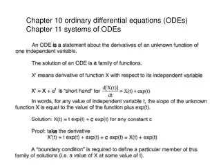
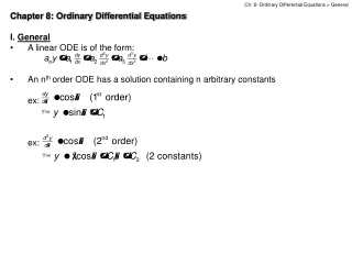
13.1 Higher Order ODEs • A higher order ODE can be converted into a system of first-order ODEs • A second-order ODE of the form can be converted to system of two first-order ODEs by a simple change of variables : the differential equations relating these variables are the initial conditions for the original ODE, become the initial conditions for the system, i.e.,
Ex.13.1 • Nonlinear pendulum Choosing g/L=1 and c/(mL)=0.3,a=π/2 and b=0. Second-order ODE-IVP Simple pendulum
13.1 Higher Order ODEs (Cont’d) • A higher order ODE may be converted to a system of first order ODEs by a similar change of variables • The nth-order ODE a system of first-order ODEs by the following change of variables; the differential equations relating these variables are with initial conditions
13.2 Systems of two first-order ODEs • 13.2.1 Euler’s method for solving two ODE-IVPs • To apply the basic Euler’s method to the system of ODEs update the function u using f(x,u,v) and update v using g(x,u,v)
Ex.13.2 • Nonlinear pendulum using Euler’s Method • To apply the basic Euler’s method In order to get accurate results, take a fairly small step, e.g., n=200 n=50 n=100 n=200 n=300
13.2 Systems of two first-order ODEs (Cont’d) • Matlab code
Ex.13.3 • Series dilution problem using Euler’s method u=c1,v=c2 u’= c’1 = -0.2u = f(x,u,v) v’= c’2 = -0.4(v-u) = g(x,u,v) n=200
13.2.2 Midpoint method for solving two ODE-IVPs • The idea is same as for Euler’s method • Update each unknown function u and v, using the basic Runge-Kutta formulas rewrite the basic second-order Runge-Kutta formulas,
13.2.2 Midpoint method for solving two ODE-IVPs • Using k1 and k2 to represent the update quantities for the unknown u • Calling the corresponding quantities for function v,m1 and m2 • Update function f by the appropriate multiple of k1 or k2 and function g by the corresponding amount of m1 or m2 • This means that k1 and m1 must be computed before k2 and m2 can be found thus,
13.2.2 Midpoint method for solving two ODE-IVPs • Matlab code
Ex.13.4 • Nonlinear pendulum using Runge-Kutta method The computed solution for n=50,n=100, and n=200 are indistinguishable n=50 n=100 n=200 n=300
Ex.13.5 • Series dilution using Runge-Kutta technique The exact solutions, viz.,
13.3 Systems of First-order ODE-IVPs • Application: chemical reactions, predator-prey models, and many others • Systems of ODEs come from the conversion of higher order ODEs into system form • Ex. 13.6 Higher Order System of ODEs • Consider the equation with initial conditions The system of ODEs is • A system of ODEs
13.3.1 Euler’s Method for Solving Systems of ODEs • The basic Euler method • The system of ODEs • Updating the function u1 using f1, u2 using f2, and u3 using f3. h is the same step size
Ex 13.8 • Solving a Higher Order System using Euler’s Method with initial conditions on [1,2] with n=2(h=0.5). at x = 3/2: at x = 2:
13.3.2 Runge-Kutta Methods for Solving Systems of ODEs • Second order Runge-Kutta method as k and m • System of three ODEs • The values of the parameter k and m • The values of unknown functions
System Using a Second-Order Runge-Kutta Method (Midpoint Method) • Matlab code function [ x, u ] = RK2_sys(f, tspan, u0, n) a = tspan(1); b = tspan(2); h = (b-a)/n; x = (a+h : h : b); k = h*feval(f, a, u0)'; m = h*feval(f, a + h/2, u0 + k/2)'; u(1, :) = u0 + m; for i = 1 : n -1 k=h*feval(f, x(i), u(i, :))'; m = h*feval(f, x(i) + h/2, u(i, :) + k/2)'; u(i+1, :) = u(i, :) + m; end x = [a x]; u = [u0, u]; The indexing of the matrix for the solution u at each step is only changed
Ex 13.9 • Solving a Higher Order System using a Runge-Kutta Method • Interval [0, 1] of the system of ODEs with initial conditions with n=2, we find the following values for x, u1, u2, and u3 • Matlab code function du = f_13_9(x, u) du = [u(2) ; u(3) ; x + 2*u(1) - 3*u(2) + 4*u(3)] [x, u] = RK2_sys('f_13_9', [0 1], [4 3 2], 2)
Ex 13.10 • Solving a Higher Order System using a Runge-Kutta Method • The electrostatic potential between two concentric spheres (radius 1 and radius 2) with initial conditions on the interval [1,2], n=2 u1(1) = 10, u2(1) = 0,u3(1) = 0, u4(1) = 1
Ex 13.10 (cont’d) The approximate solution at x = 1.5: finding k and m again
Ex 13.10 (cont’d) The approximate solution at x = 2.0: • Matlab code function du = f_13_10(x, u) du = [u(2) ; -2*u(2)/x ; u(4) ; -2*u(4)/x] [x, u] = RK2_sys('f_13_10', [1 2], [10 0 0 1],2)
Ex 13.10 (cont’d) • n = 10 • Matlab code • [x, u] = RK2_sys('f_13_10', [1 2], [10 0 0 1],10)
Fourth-Order Runge-Kutta Method • Matlab code %function f(x, u); a = tspan(1); b = tspan(2); h = (b - a)/n; x = (a+h : h : b)'; k1 = h*feval(f, a, u0)'; k2 = h*feval(f, a+h/2, u0+k1/2)'; k3 = h*feval(f, a+h/2, u0+k2/2)'; k4 = h*feval(f, a+h, u0+k3)'; u(1, :) = u0 + k1/6 + k2/3 + k3/3 + k4/6; for i = 1:n-1 k1 = h*feval(f, x(i), u(i,:))'; k2 = h*feval(f, x(i)+h/2, u(i, :)+k1/2)'; k3 = h*feval(f, x(i)+h/2, u(i, :)+k2/2)'; k4 = h*feval(f, x(i)+h, u(i, :)+k3)'; u(i+1, :) = u(i, :) + k1/6 + k2/3 + k3/3 + k4/6; end x = [a x]; u = [u0 u];
Ex 13.11 • Solving a Circular Chemical Reaction Using a Runge-Kutta Method • r1 = 0.1(t+1), r2=2, r3=1 • n = 100 • Matlab code function du = f_13_11(x, u) du = [u(3)-0.1*(x+1)*u(1) ; 0.1*(x+1)*u(1)-2*u(2) ; 2*u(2)-u(3)]; [x, u] = RK4_sys('f_13_11', [0 40], [0.8696 0.0435 0.0870], 100) nn = length(x) plot(x, u(1:nn, 1), '-',x, u(1:nn, 2),'.',x, u(1:nn, 3),'-.') A C B Concentrations of three reactants in circular chemical
13.3.3 Multistep Methods for System • The basic two-step Adams-Bashforth method • y0 is given by the initial condition • y1 is found from a one-step method, such as a Runge-Kutta • can be extended for use with a system of three ODEs u1’ = f1(x,u1,u2,u3) u2`= f2(x,u1,u2,u3) u3` = f3(x,u1,u2,u3)
13.3.3 Multistep Methods for System • The basic two-step Adams-Bashforth method (cont’d)
Adams-Bashforth-Moulton • Predictor-corrector methods • Matlab code function [x, u] = ABM3_sys(f, tspan, u0, n) a = tspan(1); b = tspan(2); h = (b-1)/n; hh = h/12; x = (a+h:h:b)'; k = h*feval(f, a, u0)'; m = h*feval(f, a+h/2, u0+k/2)'; u(1, :) = u0+m; k = h*feval(f,x(1), u(1, :))'; m = h*feval(f, x(1)+h/2, u(1,:)+k/2)'; u(2, :) = u(1, :) +m; z(2, :) = feval(f, x(2), u(2, :))'; uu(3,:) = u(2, :) + hh*(23*z(2,:) - 16*z(1, :) + 5*feval(f, a, u0)'); zz = feval(f, x(3), uu(3, :))'; u(3, :) = u(2, :) + h*(5*zz + 8*z(2, :) -z(1,:)); for i = 3:n-1 z(i, :) = feval(f, x(i), u(i, :))'; uu(i+1, :) = u(i, :) + hh*(23*z(i,:) - 16*z(i-1, :) + 5*z(i-2, :)); zz = feval(f, x(i+1), uu(i+1, :))'; u(i+1,:) = u(i,:) + hh*(5*zz + 8*z(i,:) - z(i-1,:)); end x = [a x]; u = [u0, u];
X1=0 m1 X2=0 m2 Ex 13.12 Mass-and-Spring System • The vertical displacements of two masses m1 and m2 • Spring constants s1 and s2 • Displacements x1 and x2 Initial conditions u1(0) = α1, u2(0) = α2, u3(0) = α3, u4(0) = α4
Ex 13.12 Mass-and-Spring System • Matlab code a = 0; b = 5; tspan = [a b]; n = 100; y0 = [0.5 0 0.25 0]; global s1 m1 s2 m2 s1 = 100; m1 = 10; s2 = 120; m2 = 2; r1 = 10; r2 = 15; [t, y] = ABM3_sys('f_13_12', tspan, y0, n); [nn, mm] = size(y) %out = [t y]; plot(t(1:nn), -(r1+y(1:nn, 1)), '-') hold on plot(t(1:nn), -(r2+y(1:nn, 3)), '-.') grid on plot([a b], [0 0]) hold off Displacement profiles of two masses connected by springs function du = f_13_12(t, u) global s1 m1 s2 m2 du =[u(2) ; (-s1*u(1) + s2*(u(3) – u(1)))/m1 ; u(4) ; -s2*(u(3) – u(1))/m2 ];]
Ex 13.13 Motion of a Baseball • Air resistance is one of the factors influencing how far a fly ball travels • Inital velocity of [100, 45] • Acting on the horizontal component only • Matlab code a = 0; b = 3; tspan = [a b]; n = 100; y0 = [0 100 3 45]; [t, y] = ABM3_sys('f_bb', tspan, y0, n); [nn, mm] = size(y); out = [t y]; plot(y(1:nn, 1), y(1:nn, 3), '-')
Ex 13.13 Motion of a Baseball 1. Air Resistance Proportional to Velocity in x Direction function dz = f_bb_1(x, z) dz = [z(2); -0.1*z(2) ; z(4) ; -32]; 2. Air Resistance Proportional to Velocity function dz = f_bb_2(x, z) dz = [z(2); -0.1*sqrt(z(2)^2 + z(4)^2); z(4); -32-0.1*sqrt(z(2)^2 + z(4)^2)*sign(z(4))]; 3. Air Resistance Proportional to Velocity in Squared x Direction function dz = f_bb_21(x, z) dz = [z(2); -0.0025*z(2)^2; z(4); -32]; 4. Air Resistance Proportional to Velocity Squared function dz = f_bb_22(x, z) dz = [z(2); -0.0025*(z(2)^2 + z(4)^2) z(4); -32-0.0025*(z(2)^2 + z(4)^2)*sign(z(4))]; 1 2 3 4
Stiff ODE and ILL-Conditioned Problem • Ill condition • ODE for which any error that occurs will increase, regardless of the numerical method employed • General solution is • The initial conditions • u1(0) = 3, u2(0) =-3 • We have a=0, b=3 • A component of the positive exponential will be introduced and will eventually dominate the true solution u1’ = 2u2 u2`= 2u1 u1’ = ae2x+be-2x u2`= ae2x –be-2x
Stiff ODE and ILL-Conditioned Problem • ill condition • Consider the ODE • The general solution • If we take the initial condition as y(0) = 2/ 27, the exact solution is • Any error in the numerical solution process will introduce the exponential component which will eventually dominate the true solution • Parasitic solution
Stiff ODE and ILL-Conditioned Problem • ill condition • Consider the ODE • Initial conditions u(0) = 1 , v(0)=0 • Consider the ODE • with Λ<<0 and g(t) a smooth, slowly varying function u’ = 98u + 198v v’ = -99u + 199v u(t) = 2e-t – e-100t v(t) = -e-t + e-100t
Using Matlab’s Functions • The Matlab Functions • ODE 23 • The Matlab functions for solving the ODE • [ T, Y ] = ODE(‘function_name’, tspan,x0) • ‘fuction_name’ is diffenential equations • tsapn is time duration from time t0 to tf • x0 is initial conditions • Example function f=dfuc(t,x) f=zeros(2,1); f(1) = 490/9*x(1) - 1996/9*x(2); f(2) = 12475*90*90*x(1)-49990/90*x(2); tspans=0:0.1:4; x0=[10 -20]; [t x] = ode23('dfuc',tsapns,x0);
Using Matlab’s Functions • The Matlab Functions • ODE 23 • To solve the problem of simulating the motion of a two – link planar robot arm • See Spong and Vidyasagar, Robot Dynamic and Control, John Wiley & Sons, Inc.,New York, 1989 ( p.145, ex 6.4.2) • Position, Velocity, Torques of joints • robot2 Moment of inertia for long, slender rod I1 = m1*l1^2/ 12; I2 = m2*l2^2 / 12; The Mass matrix [M] d11 = m1*Lc1^2 + m2*(L1^2 + Lc2^2 + 2*L1*Lc2*cos(r2)) + I1 + I2; d12 = m2*(Lc2^2 + L1*Lc2*cos(r2)) + I2; d21 = d12; d22 = m2*Lc2^2 + I2;
Using Matlab’s Functions • The Matlab Functions • ODE 23 • robot2_1 Plot each parameters Initialize Calculate each parameters
Using Matlab’s Functions • The Matlab Functions • ODE 23 • To solve the problem of simulating the motion of a two – link planar robot arm • robot2
Using Matlab’s Functions • The Matlab Functions • ODE 23 • Result • Figure shows the motion of the arm • Position • Velocity • Torques