Matlab statistics fundamentals
Matlab statistics fundamentals. Normal distribution % basic functions mew=100; sig=10; x=90; normpdf ( x,mew,sig ) 1/sig/ sqrt (2*pi)*exp(-(x-mew)^2/sig^2/2) x=50:150; f= normpdf ( x,mew,sig ); plot( x,f ) x=50:150; F= normcdf ( x,mew,sig ); plot( x,F ) p=0.1; norminv ( p,mew,sig )

Matlab statistics fundamentals
E N D
Presentation Transcript
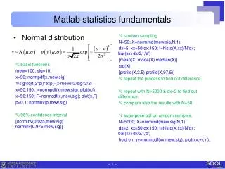
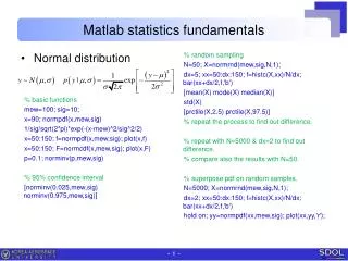
Matlab statistics fundamentals • Normal distribution • % basic functions • mew=100; sig=10; • x=90; normpdf(x,mew,sig) • 1/sig/sqrt(2*pi)*exp(-(x-mew)^2/sig^2/2) • x=50:150; f=normpdf(x,mew,sig); plot(x,f) • x=50:150; F=normcdf(x,mew,sig); plot(x,F) • p=0.1; norminv(p,mew,sig) • % 95% confidence interval • [norminv(0.025,mew,sig) norminv(0.975,mew,sig)] • % random sampling • N=50; X=normrnd(mew,sig,N,1); • dx=5; xx=50:dx:150; f=histc(X,xx)/N/dx; bar(xx+dx/2,f,'b') • [mean(X) mode(X) median(X)] • std(X) • [prctile(X,2.5) prctile(X,97.5)] • % repeat the process to find out difference. • % repeat with N=5000 & dx=2 to find out difference. • % compare also the results with N=50. • % superpose pdf on random samples. • N=5000; X=normrnd(mew,sig,N,1); • dx=2; xx=50:dx:150; f=histc(X,xx)/N/dx; bar(xx+dx/2,f,'b') • hold on; yy=normpdf(xx,mew,sig); plot(xx,yy,'r');
Matlab statistics fundamentals • Mean of normal dist. • % mean of normal distribution • mew=100; sig=10; n=10; • mean(normrnd(mew,sig,n,1)) • % repeat this to find out varying feature. • % superpose random sampling of mean • N=5000; X=normrnd(mew,sig,N,1); • dx=2; xx=50:dx:150; f=histc(X,xx)/N/dx; bar(xx+dx/2,f,'b') • Xm=mean(normrnd(mew,sig,n,N)); • dx=2; xx=50:dx:150; fm=histc(Xm,xx)/N/dx; hold on; bar(xx+dx/2,fm,'g') • % superpose pdf on random samples. • yy=normpdf(xx,mew,sig); plot(xx,yy,'r'); • yy=normpdf(xx,mew,sig/sqrt(n)); plot(xx,yy,'k'); • Interval estimation • % confidence interval of Xbar • sign=sig/sqrt(n); • [norminv(.025,mew,sign) norminv(.975,mew,sign)] • [prctile(Xm,2.5) prctile(Xm,97.5)] • [mew+norminv(.025)*sign mew+norminv(.975)*sign]
Matlab statistics fundamentals • Variance of normal dist. • % variance of normal distribution • mew=100; sig=10; n=10; • var(normrnd(mew,sig,n,1)) • % repeat this to find out varying feature. • % random sampling of variance • N=5000; S2=var(normrnd(mew,sig,n,N)); • C=(n-1)*S2/sig^2; • dc=.5; cc=0:dc:25; fc=histc(C,cc)/N/dc; bar(cc+dc/2,fc,'g') • % superpose pdf on random samples. • yy=chi2pdf(cc,n-1); hold on; plot(cc,yy,'r'); • Interval estimation • % confidence interval of variance normalized. • [chi2inv(.025,n-1) chi2inv(.975,n-1)] • [prctile(C,2.5) prctile(C,97.5)] • % confidence interval of variance • sig^2/(n-1)*[chi2inv(.025,n-1) chi2inv(.975,n-1)] • [prctile(S2,2.5) prctile(S2,97.5)]
Estimating mean with known variance • Case of single data • Consider single scalar observation y from N with unknown mean • Likelihood of y • Conjugate priorimplies that q is exponential of a quadratic form. • Posterior densityor • Posterior mean is a weighted average of prior mean m0 and observed ywith weights proportional to (inverse of variance) • If t0→ ∞ then c0→ 0, p(q) is constant over (-∞ , ∞). Then we get m1 = y, t1 = s.This means when we don’t have any knowledge on the prior distribution, we just estimate the distribution the same as the sample distribution.
Estimating mean with known variance • Case of single data • Posterior prediction • Rearrange this in terms of q to obtain • Ignore 1st term which includes q. this becomes constant after integration. Then • Mean is equal to the posterior mean.Variance has two components, predictive variance s2 and variance t12 due to posterior uncertainty in q. So, or
Estimating mean with known variance • Case of multiple data • Independent & identically distributed (iid) observations • Posterior densityOr • Posterior distribution depends on y only through the sample mean ȳ.In fact, since ȳ~N(q, s2/n), the result of single case can be applied with ȳ. • Prior precision 1/t02 and data precision n/s2 play equivalent roles.
Estimating mean with known variance • Case of multiple data • Posterior density • If there is no prior knowledge, • Let’s derive this thoroughly. • Posterior prediction (in case of no prior)
Estimating mean with known variance • Practice • 20 samples of normal distribution are given with mean 2.9 and stdev 0.2. • Plot posterior pdf of unknown population mean conditional on the observation using the analytical expression • Plot the distribution also using the simulation draw. • Superpose the two in one graph. • Plot cdf of the two together, and compute the max difference of the two.
Estimating variance with known mean • Multiple data are given. • Sample distribution where • In case of no information, the prior is • Posterior distributionThis is rewritten as • Remark • is identical to
Estimating variance with known mean • Practice • 5 samples of normal distribution are given with sample variance 0.04. • Plot posterior pdf of unknown variance conditional on the observation using the analytical expression. • Plot the distribution also using the simulation draw. • Superpose the two in one graph. • Calculate the 95% credible interval, i.e., 2.5% & 97.5% percentiles of the distribution.
Homework • To be announced.