Chapter 4 Network Layer
Chapter 4 Network Layer. Part 3: Routing. Computer Networking: A Top Down Approach 5 th edition. Jim Kurose, Keith Ross Addison-Wesley, April 2009. . 4. 1 Introduction 4.2 Virtual circuit and datagram networks 4.3 What’s inside a router 4.4 IP: Internet Protocol Datagram format

Chapter 4 Network Layer
E N D
Presentation Transcript
Chapter 4Network Layer Part 3: Routing Computer Networking: A Top Down Approach 5th edition. Jim Kurose, Keith RossAddison-Wesley, April 2009. Network Layer
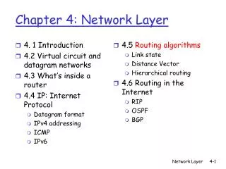
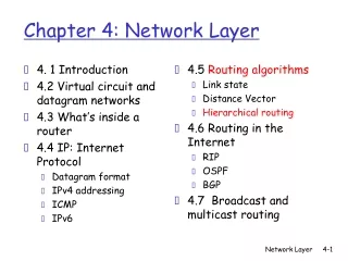
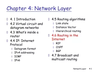
4. 1 Introduction 4.2 Virtual circuit and datagram networks 4.3 What’s inside a router 4.4 IP: Internet Protocol Datagram format IPv4 addressing ICMP IPv6 4.5 Routing algorithms Link state Distance Vector Hierarchical routing 4.6 Routing in the Internet RIP OSPF BGP 4.7 Broadcast and multicast routing Chapter 4: Network Layer Network Layer
Routing Algorithms • Need to compute the forwarding tables • Typically, a host is connected to one router (the default router or first-hop router) • We call this the source router • The default router of the destination is called the destination router • Goal: • Set of routers (nodes) • Links between routers with weights Network Layer
Routing Algorithms • Method: graph algorithm (undirected) • Graph G = (N, E) • N is set of nodes (routers) • E is collection of edges (physical links) • Represent by endpoints: (x,y) • Edges have a value representing its cost • Could be physical length • Link speed • Monetary cost • We’ll ignore what the cost represents • c(x,y) is the cost on an edge • If edge does not exist, c(x,y) = ∞ Network Layer
5 3 5 2 2 1 3 1 2 1 x z w y u v Routing Algorithms • Terminology • Path: a sequence of nodes (x1, x2, ..xp) such that each of the pairs (x1,x2), (x2,x3),…(xp-1,xp) are edges in E • Cost: sum of all edge costs along the path • Least-cost path: path between x1 and xp that has the least cost • In image, least-cost Path from u to w is (u, x, y, w) Network Layer
Routing Algorithms • Global routing algorithm • Computes the least-cost path using complete global knowledge about the network • Called link-state (LS) algorithms since it knows the ost of each link in network Network Layer
Routing Algorithms • Decentralized routing algorithm • Calculation carried out in an iterative distributed manner • No node has complete information about the costs of all network links • Each node begins with only the knowledge of the costs of its own directly attached links • Iterative process used where nodes calculate and exchange info with neighbors • Distance-vector (DV) algorithm • each node maintains a vector of estimates of the costs to all other nodes in the network Network Layer
4. 1 Introduction 4.2 Virtual circuit and datagram networks 4.3 What’s inside a router 4.4 IP: Internet Protocol Datagram format IPv4 addressing ICMP IPv6 4.5 Routing algorithms Link state Distance Vector Hierarchical routing 4.6 Routing in the Internet RIP OSPF BGP 4.7 Broadcast and multicast routing Chapter 4: Network Layer Network Layer
Dijkstra’s algorithm net topology, link costs known to all nodes accomplished via “link state broadcast” all nodes have same info computes least cost paths from one node (‘source”) to all other nodes gives forwarding table for that node iterative: after k iterations, know least cost path to k dest.’s Notation: c(x,y): link cost from node x to y; = ∞ if not direct neighbors D(v): current value of cost of path from source to dest. v p(v): predecessor node along path from source to v N': set of nodes whose least cost path definitively known A Link-State Routing Algorithm Network Layer
Dijsktra’s Algorithm 1 Initialization: (our node is u) 2 N' = {u} 3 for all nodes v 4 if v adjacent to u 5 then D(v) = c(u,v) 6 else D(v) = ∞ 7 8 Loop 9 find w not in N' such that D(w) is a minimum 10 add w to N' 11 update D(v) for all v adjacent to w and not in N' : 12 D(v) = min( D(v), D(w) + c(w,v) ) 13 /* new cost to v is either old cost to v or known 14 shortest path cost to w plus cost from w to v */ 15 until all nodes in N' Network Layer
5 3 5 2 2 1 3 1 2 1 x z w u y v Dijkstra’s algorithm: example D(v),p(v) 2,u 2,u 2,u D(x),p(x) 1,u D(w),p(w) 5,u 4,x 3,y 3,y D(y),p(y) ∞ 2,x Step 0 1 2 3 4 5 N' u ux uxy uxyv uxyvw uxyvwz D(z),p(z) ∞ ∞ 4,y 4,y 4,y Network Layer
x z w u y v destination link (u,v) v (u,x) x y (u,x) (u,x) w z (u,x) Dijkstra’s algorithm: example (2) Resulting shortest-path tree from u: Resulting forwarding table in u: Network Layer
Algorithm complexity: n nodes each iteration: need to check all nodes, w, not in N n(n+1)/2 comparisons: O(n2) more efficient implementations possible: O(nlogn) Oscillations possible: e.g., link cost = amount of carried traffic A A A A D D D D B B B B C C C C 1 1+e 2+e 0 2+e 0 2+e 0 0 0 1 1+e 0 0 1 1+e e 0 0 0 e 1 1+e 0 1 1 e … recompute … recompute routing … recompute initially Dijkstra’s algorithm, discussion Network Layer
4. 1 Introduction 4.2 Virtual circuit and datagram networks 4.3 What’s inside a router 4.4 IP: Internet Protocol Datagram format IPv4 addressing ICMP IPv6 4.5 Routing algorithms Link state Distance Vector Hierarchical routing 4.6 Routing in the Internet RIP OSPF BGP 4.7 Broadcast and multicast routing Chapter 4: Network Layer Network Layer
Distance Vector Algorithm Bellman-Ford Equation (dynamic programming) Define dx(y) := cost of least-cost path from x to y Then dx(y) = min {c(x,v) + dv(y) } where min is taken over all neighbors v of x v Network Layer
5 3 5 2 2 1 3 1 2 1 x z w u y v Bellman-Ford example Clearly, dv(z) = 5, dx(z) = 3, dw(z) = 3 B-F equation says: du(z) = min { c(u,v) + dv(z), c(u,x) + dx(z), c(u,w) + dw(z) } = min {2 + 5, 1 + 3, 5 + 3} = 4 Node that achieves minimum is next hop in shortest path ➜ forwarding table Network Layer
Distance Vector Algorithm • Dx(y) = estimate of least cost from x to y • Node x knows cost to each neighbor v: c(x,v) • Node x maintains distance vector Dx = [Dx(y): y є N ] • Node x also maintains its neighbors’ distance vectors • For each neighbor v, x maintains Dv = [Dv(y): y є N ] Network Layer
Distance vector algorithm (4) Basic idea: • From time-to-time, each node sends its own distance vector estimate to neighbors • Asynchronous • When a node x receives new DV estimate from neighbor, it updates its own DV using B-F equation: Dx(y) ← minv{c(x,v) + Dv(y)} for each node y ∊ N • Under minor, natural conditions, the estimate Dx(y) converge to the actual least costdx(y) Network Layer
Iterative, asynchronous: each local iteration caused by: local link cost change DV update message from neighbor Distributed: each node notifies neighbors only when its DV changes neighbors then notify their neighbors if necessary wait for (change in local link cost or msg from neighbor) recompute estimates if DV to any dest has changed, notify neighbors Distance Vector Algorithm (5) Each node: Network Layer
cost to x y z x 0 2 7 y from ∞ ∞ ∞ z ∞ ∞ ∞ 2 1 7 z x y Dx(z) = min{c(x,y) + Dy(z), c(x,z) + Dz(z)} = min{2+1 , 7+0} = 3 Dx(y) = min{c(x,y) + Dy(y), c(x,z) + Dz(y)} = min{2+0 , 7+1} = 2 node x table cost to x y z x 0 2 3 y from 2 0 1 z 7 1 0 node y table cost to x y z x ∞ ∞ ∞ 2 0 1 y from z ∞ ∞ ∞ node z table cost to x y z x ∞ ∞ ∞ y from ∞ ∞ ∞ z 7 1 0 time Network Layer
cost to x y z x 0 2 7 y from ∞ ∞ ∞ z ∞ ∞ ∞ 2 1 7 z x y Dx(z) = min{c(x,y) + Dy(z), c(x,z) + Dz(z)} = min{2+1 , 7+0} = 3 Dx(y) = min{c(x,y) + Dy(y), c(x,z) + Dz(y)} = min{2+0 , 7+1} = 2 node x table cost to cost to x y z x y z x 0 2 3 x 0 2 3 y from 2 0 1 y from 2 0 1 z 7 1 0 z 3 1 0 node y table cost to cost to cost to x y z x y z x y z x ∞ ∞ x 0 2 7 ∞ 2 0 1 x 0 2 3 y y from 2 0 1 y from from 2 0 1 z z ∞ ∞ ∞ 7 1 0 z 3 1 0 node z table cost to cost to cost to x y z x y z x y z x 0 2 7 x 0 2 3 x ∞ ∞ ∞ y y 2 0 1 from from y 2 0 1 from ∞ ∞ ∞ z z z 3 1 0 3 1 0 7 1 0 time Network Layer
1 4 1 50 x z y Distance Vector: link cost changes Link cost changes: • node detects local link cost change • updates routing info, recalculates distance vector • if DV changes, notify neighbors At time t0, y detects the link-cost change, updates its DV, and informs its neighbors. “good news travels fast” At time t1, z receives the update from y and updates its table. It computes a new least cost to x and sends its neighbors its DV. At time t2, y receives z’s update and updates its distance table. y’s least costs do not change and hence y does not send any message to z. Network Layer
60 4 1 50 x z y Distance Vector: link cost changes Link cost changes: • good news travels fast • bad news travels slow - “count to infinity” problem! • Assume cost between x and y increases from 4 to 60 • Before link cost changes Dy(x) = 4, Dy(z) = 1, Dz(y) = 1, Dz(x) = 5. Network Layer
60 4 1 50 x z y Distance Vector: link cost changes • 1. At time t0 y detects the link-cost change. Computes new min-cost path to x of: • Dy(x) = min{c(y,x)+Dx(x), c(y,z) + Dz(x)} • = min{60 + 0, 1 + 5} = 6 • We know this is wrong; but y only knows that c(y,x) = 60 and that z could get to x with cost of 5. • Routing loop: in order to get to x, y goes through z and z routes through y. • A packet will bounce back and forth between y and z forever! 2. Since node y has computed a new min cost to x, it informs z of its new distance vector at time t1 3. z receives y’s new DV which indicates that y’s min cost to x is 6. z computes new distance vector with Dz(x) = min {50 + 1, 1 + 6} = 7. z’s DV has changed, so it notifies y at time t2 Now y receives z’s new DV, so it recalc, determines Dy(z) = 8, etc. Takes 44 iterations!! Network Layer
60 4 1 50 x z y Distance Vector: link cost changes Poisoned reverse: • If Z routes through Y to get to X : • Z tells Y its (Z’s) distance to X is infinite (so Y won’t route to X via Z) • Z continues to tell this lie as long as it routes to x via y • will this completely solve count to infinity problem? • No…loops involving 3 or more nodes will not be detected by the poisoned reverse technique Network Layer
Message complexity LS: with n nodes, E links, O(nE) msgs sent DV: exchange between neighbors only convergence time varies Speed of Convergence LS: O(n2) algorithm requires O(nE) msgs may have oscillations DV: convergence time varies may be routing loops count-to-infinity problem Robustness: what happens if router malfunctions? LS: node can advertise incorrect link cost each node computes only its own table DV: DV node can advertise incorrect path cost each node’s table used by others error propagate thru network Comparison of LS and DV algorithms Network Layer
LS and DV algorithms • Are essentially the only algorithms used in practice in the intenet. • Lots of theoretical work done on algorithms Network Layer
4. 1 Introduction 4.2 Virtual circuit and datagram networks 4.3 What’s inside a router 4.4 IP: Internet Protocol Datagram format IPv4 addressing ICMP IPv6 4.5 Routing algorithms Link state Distance Vector Hierarchical routing 4.6 Routing in the Internet RIP OSPF BGP 4.7 Broadcast and multicast routing Chapter 4: Network Layer Network Layer
scale: with 200 million destinations: can’t store all dest’s in routing tables! routing table exchange would swamp links! LS message would swamp the net! DV would never converge! administrative autonomy internet = network of networks each network admin may want to control routing in its own network Hierarchical Routing Our routing study thus far - idealization • all routers identical • network “flat” … not true in practice Network Layer
aggregate routers into regions, “autonomous systems” (AS) An AS is a group of routers under the same admin control (e.g., same ISP) routers in same AS run same routing protocol Called the “intra-AS” routing protocol routers in different AS can run different intra-AS routing protocol Gateway router Direct link to router in another AS Hierarchical Routing Network Layer
forwarding table configured by both intra- and inter-AS routing algorithm intra-AS sets entries for internal dests inter-AS & intra-As sets entries for external dests 3a 3b 2a AS3 AS2 1a 2c AS1 2b 3c 1b 1d 1c Inter-AS Routing algorithm Intra-AS Routing algorithm Forwarding table Interconnected ASes AS1, AS2, AS3 could run different routing algms If there is only one connection to outside net, routing between Ases is easy Routers 1b, 1c, 2a, 3a are gateway routers Network Layer
AS1 must: learn which dests are reachable through AS2, which through AS3 propagate this reachability info to all routers in AS1 Job of inter-AS routing! suppose router in AS1 receives datagram destined outside of AS1: router should forward packet to gateway router, but which one? 3a 3b 2a AS3 AS2 1a AS1 2c 2b 3c 1b 1d 1c Inter-AS tasks Network Layer
2c 2b 3c 1b 1d 1c Example: Setting forwarding table in router 1d • suppose AS1 learns (via inter-AS protocol) that subnet x reachable via AS3 (gateway 1c) but not via AS2. • inter-AS protocol propagates reachability info to all internal routers. • router 1d determines from intra-AS routing info that its interface I is on the least cost path to 1c. • installs forwarding table entry (x,I) … x 3a 3b 2a AS3 AS2 1a AS1 Network Layer
3a 3b 2a AS3 AS2 1a AS1 2c 2b 3c 1b 1d 1c Example: Choosing among multiple ASes • now suppose AS1 learns from inter-AS protocol that subnet x is reachable from AS3 and from AS2. • to configure forwarding table, router 1d must determine towards which gateway it should forward packets for dest x. • this is also job of inter-AS routing protocol! … … x Network Layer
Determine from forwarding table the interface I that leads to least-cost gateway. Enter (x,I) in forwarding table Use routing info from intra-AS protocol to determine costs of least-cost paths to each of the gateways Learn from inter-AS protocol that subnet x is reachable via multiple gateways Hot potato routing: Choose the gateway that has the smallest least cost Example: Choosing among multiple ASes • now suppose AS1 learns from inter-AS protocol that subnet x is reachable from AS3 and from AS2. • to configure forwarding table, router 1d must determine towards which gateway it should forward packets for dest x. • this is also job of inter-AS routing protocol! • hot potato routing: send packet towards closest of two routers. Network Layer
4. 1 Introduction 4.2 Virtual circuit and datagram networks 4.3 What’s inside a router 4.4 IP: Internet Protocol Datagram format IPv4 addressing ICMP IPv6 4.5 Routing algorithms Link state Distance Vector Hierarchical routing 4.6 Routing in the Internet RIP OSPF BGP 4.7 Broadcast and multicast routing Chapter 4: Network Layer Network Layer
Intra-AS Routing • also known as Interior Gateway Protocols (IGP) • most common Intra-AS routing protocols: • RIP: Routing Information Protocol • OSPF: Open Shortest Path First • IGRP: Interior Gateway Routing Protocol (Cisco proprietary) Network Layer