Download
1 / 14
140 likes | 284 Vues
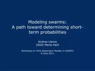
Modeling swarms: A path toward determining short-term probabilities. Andrea Llenos USGS Menlo Park Workshop on Time-Dependent Models in UCERF3 8 June 2011. Outline. Motivation: Why are swarms important for UCERF? Where things stand now Characteristics of swarms

E N D
Modeling swarms:A path toward determining short-term probabilities Andrea Llenos USGS Menlo Park Workshop on Time-Dependent Models in UCERF3 8 June 2011
Outline • Motivation: Why are swarms important for UCERF? • Where things stand now • Characteristics of swarms • Detecting swarms (retrospectively) • What needs to be done • Detecting swarms (prospectively) • Implementation • As ETAS add-on? • As a data assimilation application? Observed seismicity rate Background seismicity rate Aftershock sequences
Time-dependent background rates are needed to account for rate changes due to external (aseismic) processes 2000 Izu Islands swarm (magma/fluids) 2000 Vogtland/Bohemia swarm (fluids) Hainzl and Ogata (2005) Lombardi et al. (2006) 2003-2004 Ubaye swarm (fluid-flow) Daniel et al. (2011)
Salton Trough Time-dependent background rate matches observed seismicity better than stationary ETAS model Transformed Time Llenos and McGuire (2011)
Characteristics of swarms • Increase in seismicity rate above background without clear mainshock • Don’t follow empirical aftershock laws • Bath’s Law • Omori’s Law • These characteristics make them appear anomalous to ETAS Holtkamp and Brudzinski (2011)
Detecting swarms in an earthquake catalog Swarms associated with aseismic transients 2005 Obsidian Buttes, CA (1985-2005, SCEDC) 2005 Kilauea, HI (2001-2007, ANSS) 2002, 2007 Boso, Japan (1992-2007, JMA) Slow slip events on the subduction plate interface off of Boso, Japan observed by cGPS, tiltmeter Shallow aseismic slip on a strike-slip fault in southern CA observed by InSAR and GPS Lohman & McGuire (2007) Slow slip events on southern flank of Kilauea volcano in HI observed by GPS Wolfe et al. (2007) Ozawa et al. (2007)
Data analysis: ETAS model optimization Swarms associated with aseismic transients 2005 Obsidian Buttes, CA (1985-2005, SCEDC) 2005 Kilauea, HI (2001-2007, ANSS) 2002, 2007 Boso, Japan (1992-2007, JMA) • Optimize ETAS model to fit catalog prior to swarm and extrapolate fit through remainder of catalog • Calculate transformed times (~ ETAS predicted number of events in a time interval) • Cumulative number of events vs. transformed time should be linear if seismicity behaving as a point process • Positive deviations occur when more seismicity is being triggered in a time interval than ETAS can explain 2005 Kilauea
Swarms appear as anomalies relative to ETAS 2005 Obsidian Buttes 2002, 2007 Boso, Japan 2005 Kilauea
A path toward determining short-term probabilities • Build off of ETAS-based forecasts • Detect that a swarm is occurring • Has been done retrospectively • Prospectively? • During the swarm • Re-estimate the background rate (and other parameters?) • Re-calculate short-term probabilities • How often? 1x? 2x? Every 5 days? 10 days? • Identify when the swarm is over • Return to pre-swarm background rate? • More sophisticated approaches (e.g., data assimilation)?
Data Assimilation Algorithms • Combines dynamic model with noisy data (e.g. seismicity rates) to estimate the temporal evolution of underlying physical variables (states) • Examples: Kalman filters, particle filters • Applications in navigation, tracking, hydrology Welch & Bishop (2001)
Data Assimilation Example • State-space model based on rate-state equations • States: stressing rate, rate-state state variable g • Algorithm: Extended Kalman Filter • Approach: Optimize ETAS for the catalog, subtract ETAS predicted aftershock rate to obtain time-dependent background rate, use data assimilation algorithm to estimate stressing rate and detect transients that trigger swarms Llenos and McGuire (2011)
A path toward determining short-term probabilities • Build off of ETAS-based forecasts • Detect that a swarm is occurring • Has been done retrospectively • Prospectively? • During the swarm • Re-estimate the background rate (and other parameters?) • Re-calculate short-term probabilities • How often? 1x? 2x? Every 5 days? 10 days? • Identify when the swarm is over • Return to pre-swarm background rate? • More sophisticated approaches (e.g., data assimilation)?
Outline • Why are swarms important for UCERF? • Need time-dependent background rate (mu) to model earthquake rates observed in catalogs accurately • Salton Trough • Ubaye France • CampeiFlagrei • Vogtland Bohemia • Swarms prevalent in Salton Trough, volcanic regions like Long Valley, places where M>6 events have occurred • Characteristics of swarms • Don’t fit empirical models of aftershock clustering, appear anomalous • ETAS parameters change during swarms (primarily stationary background rate) • How to implement this to calculate short-term probabilities? • Where we are now • Detection (retrospective) • How they affect ETAS parameters • Outstanding issues that need to be addressed • Data assimilation?